L04 Credit Risk Management

L04 Credit Risk Management

Introduction to Credit Risk

Settlement Risk

Credit risk is the risk of an economic loss from the failure of a couterparty to fulfill its contractual obligations.
- its effect is measured by the cost of replacing cash flow if the other party defaults
- it requires constructing the distribution of default probabilities, of loss given default (LGD), and of credit exposures
- traditionally, it is viewed as **presettlement risk, which arises during the life of the obligation
Presettlement risk is the risk of loss due to the counterparty's failure to perform on an obligation during the life of the transaction
- it includes the default on a loan or bond or failure to make required payment on a derivative transaction
- it exists over long periods
Settlement risk is due to the exchange of cash flow and is of a much shorter-term nature
- it arises as soon as an institution makes the required payment and exists until the offsetting payment is received
- the risk is greatest when payments occur in different time zones, especially for foreign exchange transactions where notional are exchanged in different currencies
- it can be caused by counterparty default, liquidity constraints, or operational problems
Status of a trade
- Revocable: When the institution can still cancel the transaction without the consent of the counterparty
- Irrevocable: After the payment has been sent and before payment from the other party is due
- Uncertain: After the payment from the other party is due but before it is actually received
- Settled: After the counterparty payment has been received
- Failed: After it has been established that the counterparty has not made the payment
Settlement risk occurs during the period of irrevocable and uncertain status (one to three days)
Tools for settlement risk management
- real-time-gross settlement (RTGS) system
- netting agreements (bilateral netting, multilateral netting system / continuous-linked settlements )
- contract for differences (CFDs)

Overview of Credit Risk

Drivers of Credit Risk

Credit risk measurement systems attempt to quantify the risk of losses due to counterparty default
- probability of default (PD)
- credit exposure (CE)
- loss given default (LGD) or recovery rate
The borrower has the option to default, so the payment pattern is exactly equivalent to a short position in an option
$CE_t=\max(V_t,0)$

Measurement of Credit Risk

Measurement of Credit Risk
- Notional amounts, adding up simple exposures
- Risk-weighted amounts, adding up exposures with a rough adjustment for risk
- Notional amounts combined with credit rating, adding up exposures adjusted for default probabilities
- Internal portfolio credit models, integrating all dimensions of credit risk
Credit Risk versus Market Risk

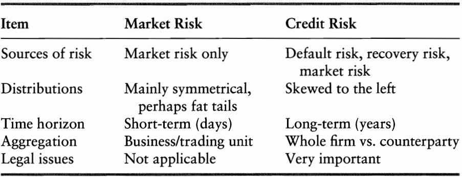
Measuring Credit Risk

Credit Losses

Default mode: suppose all losses are due to the effect of defaults only.

The distribution of cresit losses (CLs) from a portfolio of $N$ instruments issued by different obligators can be described as
$CL=\sum_{i=1}^Nb_i\times CE_i\times(1-f_i)$

If $b$ , $CE$ and $f$ are all independent, he expected credit loss is
$E[CL]=\sum_{i=1}^NE[b_i]\times E[CE_i]\times E[LGD_i]=\sum_{i=1}^Np_i\times E[CE_i]\times E[LGD_i]$

If assuming $CE_i=\$1$ for all $i=1,2,\dots,n$ , we have
$E{CL}=E\left[\sum_{i=1}^nLGD_i\right]=E[n]E[LGD]=npE[LGD]$
The variance can be derived using the following formula
$V[CL]=E\left\{V[CL|n]\right\}+V\left\{E[CL|n]\right\}=E\left\{nV[LGD]\right\}+V\left\{nE[LGD]\right\}$
So we have
$\begin{array}{lll} V[CL]&=&E[n]V[LGD]+v[n]\{E[LGD]^2\}\\ &=&NpV[LGD]+Np(1-p)\{E[LGD]^2\} \end{array}$
When $N=1$ , the standard deviation is
$SD[CL]=\sqrt{pV[LGD]+p(1-p)\{E[LGD]^2\}}$

Measuring Actuarial Default Risk

Credit Event

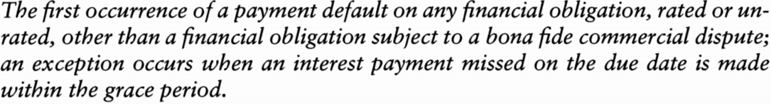
Definition of default by Standard & Pool's

Definition of credit event by International Swaps and Derivatives Association (ISDA)

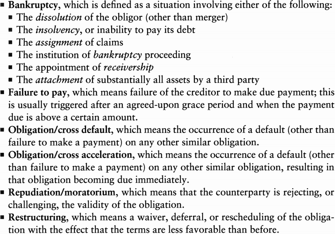
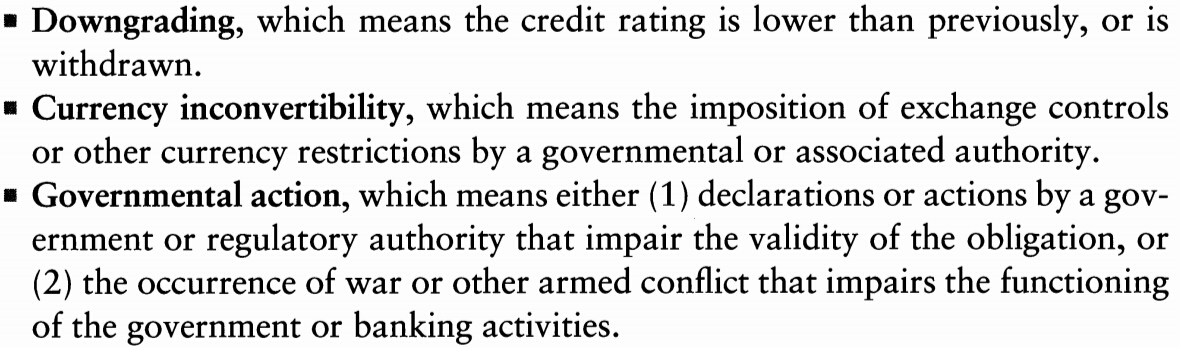
Other events sometimes included are

Default Rates

Credit Ratings

A credit rating is an ''evaluation of creditworthiness'' issued by a credit rating agency (CRA).
The major U.S. bond rating agencies are
- Moody's Investors Service
- Standard and Pool's (S&P)
- Fitch Ratings
Moody's definition of a credit rating
Ratings represent objective (or actuarial) probabilities of default
- published default frequencies can be used to convert ratings to default probabilities

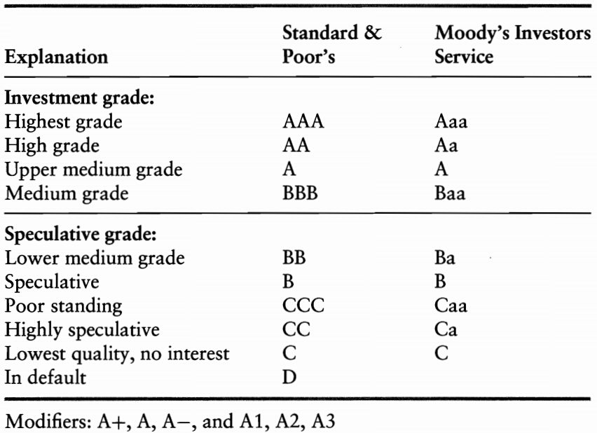
Ratings
- investment grade
- speculative grade, or below investment grade
Classes & modifiers (also called notches)

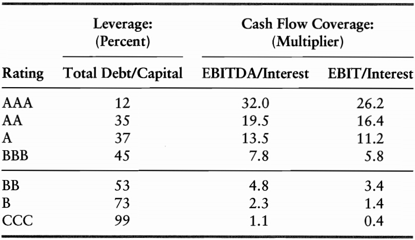
Accounting ratios & credit ratings
Multiple Discriminant Analysis (MDA)
- MDA constructs a linear combination of accounting data that provides the best fit with the observed states of default and non-default for the sample firms
- $z-$ score is an example of MDA
$z-$ score (Altman, 1968), variable used are:
- $X_1$ : working capital over other assets,
- $X_2$ : retained earnings over total assets,
- $X_3$ : EBIT over total assets,
- $X_4$ : market value of equity over total liabilities,
- $X_5$ : net sales over total assets.
  $Z=1.2X_1+1.4X_2+3.3X_3+0.6X_4+0.999X_5$

$z-$ score	$<1.8$	$1.8\sim2.7$	$2.7\sim3.0$	$>3.0$
implications	very likely to default	good chance of default	on alert	unlikely to default

Historical Default Rates

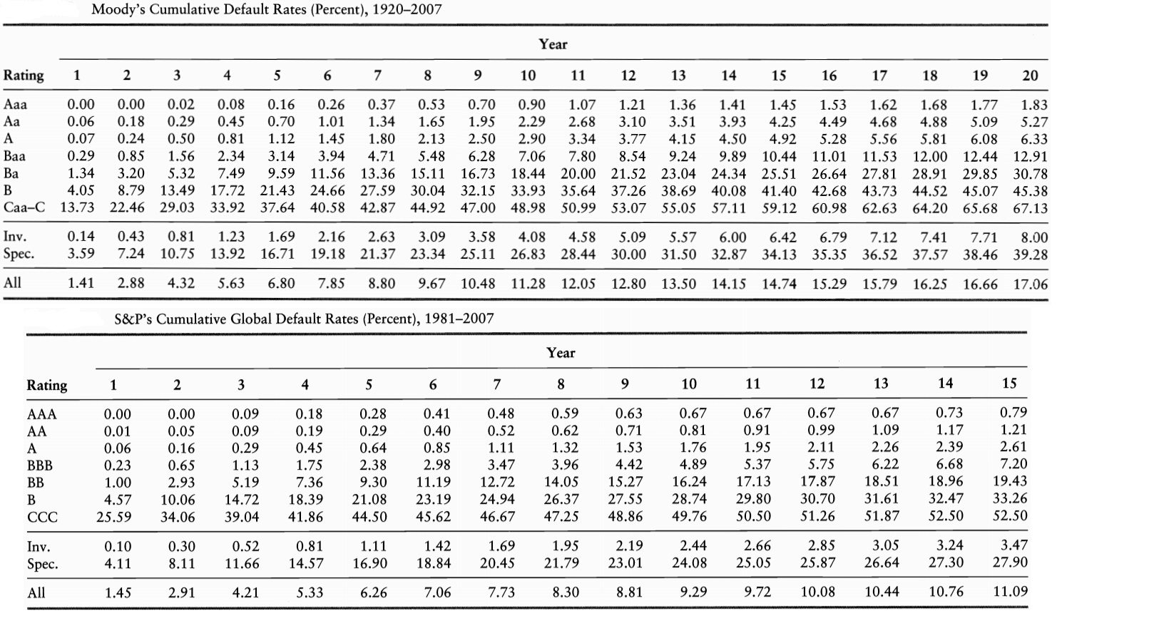
The standard deviation of default probability (about 0.01%) for AA-rated credits is on the same of as the average (0.01%)
Estimation of default rates for low probability events can be very imprecise

Cumulative and Marginal Dafault Rates

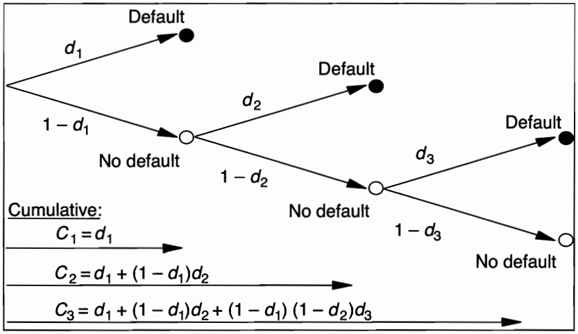
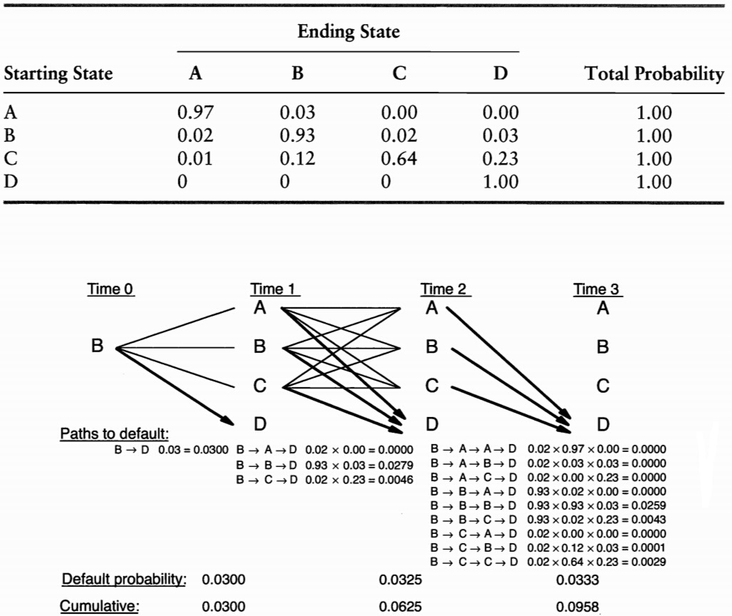
Cumulative default rates measure the total frequency of default at any time between the starting date and year $T$ , while marginal default rates measure default during year $T$
Notations
- $m[t+N|R(t)]$ : the number of issuers rated $R$ at the end of year $t$ that default in year $T=t+N$
- $n[t+N|]$ : the number of issuers rated $R$ at the end of year $t$ that have not default by the beginning of year $T=t+N$
Calculating rates
- Marginal Default Rate during Year $T$ : $d_N(R)=\frac{m[t+N|R(t)]} {n[t+N|R(t)]}$
- Survival Rate: $S_N(R)=\prod_{i=1} ^N(1-d_i(R))$
- Marginal Default Rate from Start to Year $T$ : $k_N(R)=S_{N-1} (R)d_N(R)$
- Cumulative Default Rate: $C_N(R)=k_1(R)+k_2(R)+\cdots+k_N(R)=1-S_N(R)$
- Average Default Rate: $C_N=1-\prod_{i=1} ^N(1-d_i)=1-(1-d)^N$
- Average Default Rate for different compounding frequencies:
  $C_N=1-(1-d^a)^N=1-(1-d^s/2)^{2N} \rightarrow1-e^{-d^cN}$

Transition Probabilities

Recovery Rates

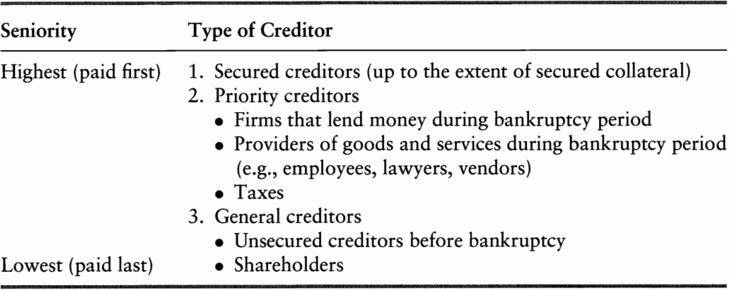
The Bankruptcy Processes

Pecking order for a company's creditor:

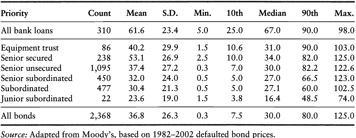
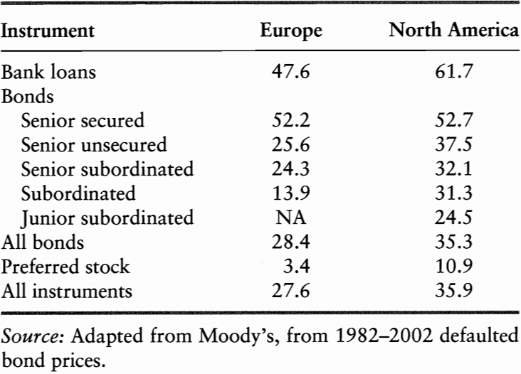
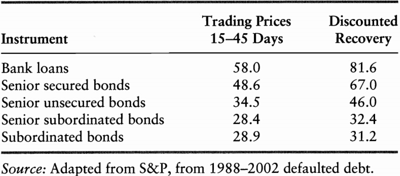
Estimates of Recovery Rates

The recovery rate depends on the following factors:

The recovery rate for corporate debt.

The legal environment is also a main driver of recovery rates.

Trading prices of debt shortly after default can be used as an estimator of recovery rate, however, they are on average lower than the discounted recovery rates
- clienteles for the two markets are different
- risk premium in trading price
An opportunity: buying the defaulted debt and working through the recovery process should create value
- distress securities funds

Measuring Default Risk from Market Prices

Corporate Bond Prices

Spreads and Default Risk: Single Period

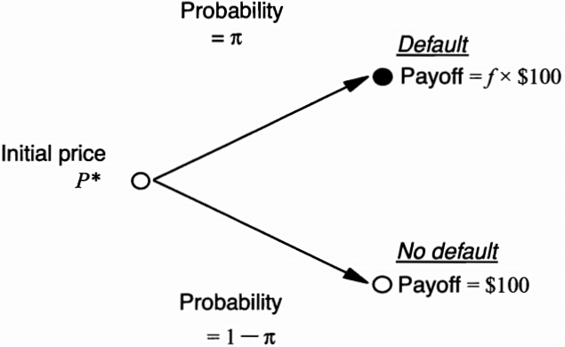
Suppose a bond has a single payment $100 in one period, the market-determined yield $y^*$ can be derived from its price $P^*$
$P^*=\frac{\$100} {(1+y^*)}$
We apply risk-neutral pricing:

$P^*=\frac{\$100} {(1+y^*)} =\left[\frac{\$100 }{(1+y)} \right]\times(1-\pi)+\left[\frac{f\times\$100 }{(1+y) }\right]\times\pi$
$\Longrightarrow(1+y)=(1+y^*)[1-\pi(1-f)]\Longrightarrow\pi=\frac{1 }{1-f} \left[1-\frac{1+y }{1+y^*} \right]\Longrightarrow y^*\approx y+\pi(1-f)$

Spreads and Default Risk: Multiple Periods

We compound interest rates and default rates over each period.Let $\pi^a$ be the average annual default rate.
$P^*=\frac{\$100 }{(1+y^*)^T} =\left[\frac{\$100} {(1+y)^T }\right]\times(1-\pi^a)^T+\left[\frac{f\times\$100} {(1+y)^T }\right]\times[1-(1-\pi^a)^T]$
$\Longrightarrow(1+y)^T=(1+y^*)^T\{(1-\pi^a)^T+f[1-(1-\pi^a)^T]\}$
If we use the cumulative default probability
$\frac{1} {(1+y^*)^T} =\left[\frac{1} {(1+y)^T} \right]\times(1-\pi)+\left[\frac{f\times1} {(1+y)^T} \right]\times[1-(1-\pi)]$
A very rough approximation:
$\Longrightarrow\frac{1 }{(1+y^*)^T} =\left[\frac{1} {(1+y)^T} \right]\times[1-\pi(1-f)]\Longrightarrow y^*\approx y+(\pi/T)(1-f)$

Risk Premium

In the previous analysis we assume risk neutrality. As a result, $\pi$ is a risk neutral measure, which is not necessarily equal to the objective, physical probability of default.

Assuming $\pi'$ and $y'$ be the physical probability of default and the discount rate. We have the following

$P^*=\frac{\$100} {(1+y^*)} =\left[\frac{\$100} {(1+y')} \right]\times(1-\pi')+\left[\frac{f\times\$100} {(1+y')} \right]\times\pi'$

$\Longrightarrow y^*\approx y+\pi'(1-f)+rp$

The risk premium ( $rp$ ) must be tied to some meaure of bond riskiness as well as investor risk aversion. In addition, this premium may incorporate a **liquidity premium and tax effects.

Cross-Section of Yield Spreads

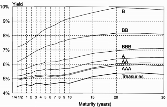
The transition from Treasuries to AAA credit most likely reflects other factors, such as liquidity and tax effects, rather than actuarial credit risk
We can use information in corporate bond yield to make inferences about credit risk
Movements in corporate bond prices tend to \textit{lead changes in credit ratings

Time Variation in Credit Spreads

Part of default risk can be attributed to common credit risk factors such as

General Economic conditions
- growth
- slow down
Volatility
- investors require more risk premium in a more volatile environment
- liquidity may dry up
The effect of volatility through an option channel
- a callable bond = bond + (short) a call
- the value of call increases in a more volatile environment

Equity Prices

The Merton Model

The Merton (1974) model views equity as akin to a call option on the assets of the firm, with an exercise price given by the face value of debt
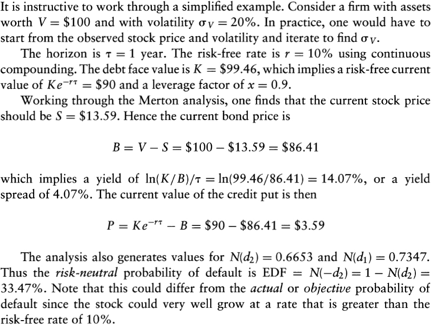
Consider a firm with total value $V$ that has one bond due in one period with face value $K$
- equity can be viewed as a call option on the firm value with strike price equal to the face value of debt
  $S_T=\max(V_T-K,0)$
- the current stock price embodies a forecast of default probability in the same way that an option embodies a forecast of being exercised
- corporate debt can be viewed as risk-free debt minus a put option on the firm value
  $B_T=V_T-S_T=\min(V_T,K)=K-\max(K-V_T,0)$

Pricing Equity and Debt

Firm value follows the geometric Brownian motion
$dV=\mu Vdt+\sigma vdz$
The value of firm can be decompose in to the value of equity ( $S$ ) and the value of debt ( $B$ ). The corporate bond price is obtained as
$B=F(V,t),\text{ }F(V,T)=\min(V,B_F),\text{ }B_F=K$
The equity value is
$S=f(V,t),\text{ }f(V,T)=\max(V-B_F,0)$

Stock Valuation
$S=\text{Call}=VN(d_1)-Ke^{-r\tau}N(d_2)$
where $d_1=\frac{\ln(V/Ke^{-r\tau})}{\sigma\sqrt{\tau}}+\frac{\sigma\sqrt{\tau}}{2},\text{ }d_2=d_1-\sigma\sqrt{\tau}$

Firm Volatility
$\sigma_V=(1/\Delta)\sigma_S(S/V)$

Bond Valuation
$B=\text{Risk-free bond}-\text{Put}\Longrightarrow B/Ke^{-r\tau}=N(d_2)+(V/Ke^{-r\tau})N(-d_2)$

Risk-Neutral Dynamics of Default
$1-N(d_2)=N(-d_2)$

Pricing Credit Risk
$\text{PD}=N[z]=N\{[\ln(K/V)-\delta\tau+0.5\sigma^2\tau]/[\sigma\sqrt{\tau}]\}$

Credit Option Valuation
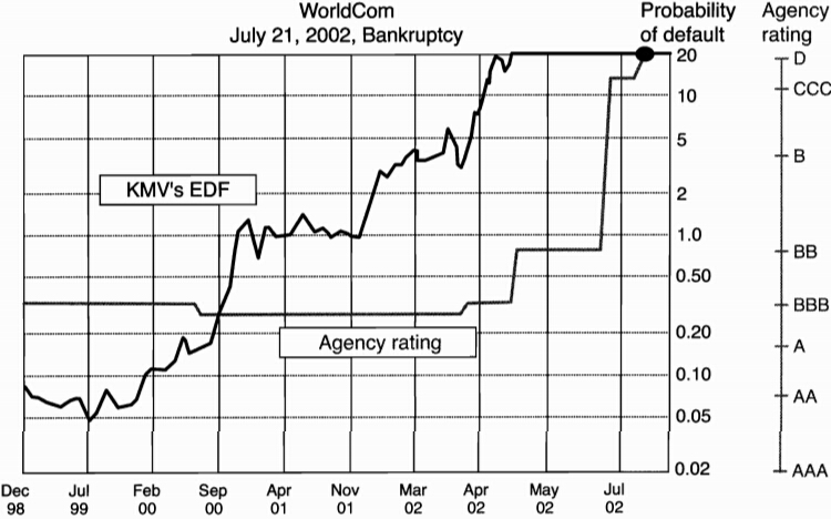
$\text{Put}=Ke^{-r\tau}-\{Ke^{-r\tau}N(d_2)+V[1-N(d_1)]\}=-V[N(-d_1)]+Ke^{-r\tau}[N(-d_2)]$

Applying the Merton Model

the KMV approach**: the company sells expected default frequencies (EDFs) for global firms
Advantages
- it relies on the price of equities, which are more actively traded than bonds
- correlations between equity prices can generate correlations between bonds
- it generates movements in EDFs that seems to \textit{lead changes in credit ratings

Disadvantages
- it can not be used to price sovereign credit risk
- it relies on a static model of the firm's capital and risk structure
- management could undertake new projects that increases not only the value if equity but also its volatility
- the model fails to explain the magnitude of credit spreads we observe on credit-sensitive bonds

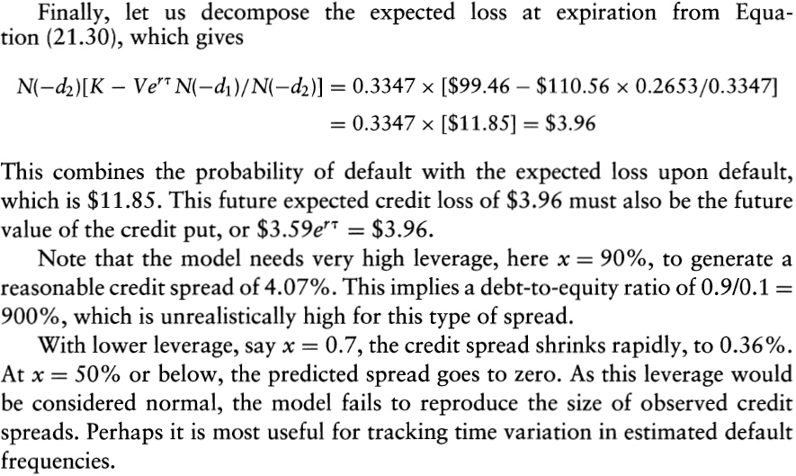
A Detailed Example

课堂练习

假设某3年期企业债券每年支付7%的券息，每半年付息一次，收益率为5%（以每半年复利计）。所有期限的无风险债券的收益率均为4%（以每半年复利计）。假设违约事件可能每半年发生一次（刚好在债券每次付息之前），回收率为45%。请在以下假设下估计违约概率：

在每个可能违约的日期，无条件违约概率均相同；
在每个可能违约的日期之前无违约的条件下，发生违约条件概率均相同。

课堂练习

请根据以下条件分析债券的违约概率和到期收益率：

无风险利率为每年4%，某信用债券的收益率为每年6%。假设若该债券违约，回收率为70%。请估计该债券一年内发生违约的概率为多少？；
某风险分析师尝试估计一个BB级债券的收益率。如果无风险利率为每年3.5%，BB级债券的违约概率为7%，违约损失率(Loss given default)为70%。请估计该债券的到期收益率。

Credit Exposures

Credit Exposore by Instrument

Credit exposure: $CE_t=\max(V_t,0)$
- current exposure is the value of the asset at the current time $V_t$ if possitive
- potential exposure represents the exposure on some future date, or set of dates
Loans or Bonds
- loans or bonds are balance sheet assets whose current and potential exposure basically is notional, or amount lent or invested
- the exposure is also notional for receivables and trade credits, as the potential loss is the amount due
Garantees
- guarantees are off-balance-sheet contracts whereby the bank has underwritten, or agrees to assume, the obligations of a third party.
- the exposure is the notional amount
- it is irrevocable
Commitments
- Commitments are off-balance-sheet contracts whereby the bank commits to a future transaction that may result in creating a credit exposure at a \textit{future date
- **irrevocable commitments vs. **revocable commitments
Swaps or Forwards
- Swaps or forwards contracts are off-balance-sheet items that can be viewed as irrevocable commitments to purchase or sell some asset on prearranged terms
- the current and potential exposure will vary from zero to a large amount depending on movements in the driving risk factors
- similar arrangement are **sale-repurchase (repos)
Long Options
- Options are off-balance-sheet items that may create many credit exposure
- the current and potential exposure will vary from zero to a large amount depending on movements in the driving risk factors
- there is no possibility for options to have negative values
Short Options
- the current and potential exposure for short options is zero because the bank writting the option can incur only a negative cash flow, assuming the option premium has been fully paid

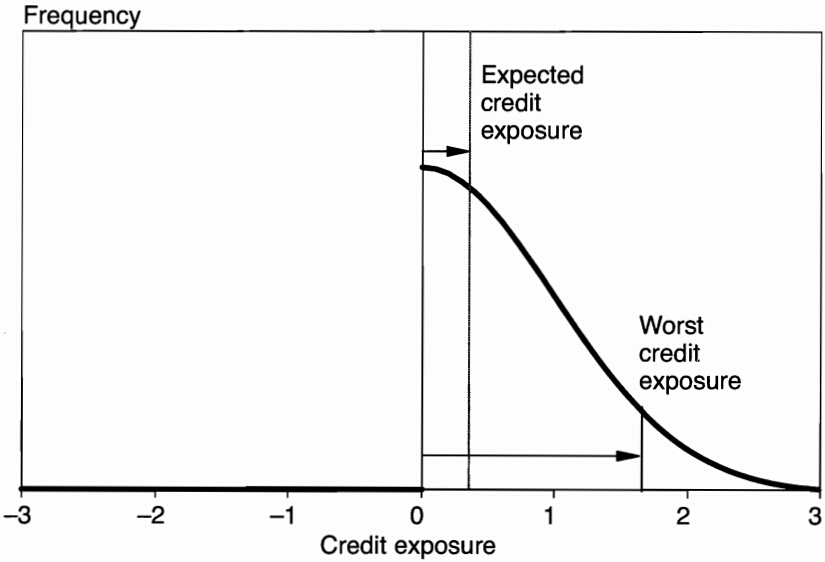
Distribution of Credit Exposure

Expected & Worse Exposure

The expected credit exposure (ECE) is the expected value of the asset replacement value $x$ , if positive, on a target date:
$\text{ECE}=\int_{-\infty}^{\infty}x^+f(x)dx$

The worse credit exposure (WCE) is the largest (worst) credit exposure at some level of confidence. It is implicitly defined as the value that is not exceeded at the given confidence level $p$ :
$1-p=\int_{\text{WCE}}^{\infty}f(x)dx$

To model the potential credit exposure, we need to

model the distribution of risk factors
evaluate the instrument given these risk factors
the process is identical to a market value at risk computation
the aggregation takes place at the counterparty level if contracts are netted

Time Profile

The average expected credit exposure (AECE) is the average of the expected credit exposure over time, from now to maturity $T$ :

$\text{AECE}=\frac{1}{T}\int_{t=0}^T\text{ECE}_tdt$

The average worst credit exposure (AWCE) is defined similarly:

$\text{AWCE}=\frac{1}{T}\int_{t=0}^T\text{WCE}_tdt$

Exposure Modifiers

Marking-to-Market (MTM)

involves settling the variation in the contract value on a regular basis
- it is called two-way marking to market if the treatment is symmetrical across the two counterparties
- if one party settles losses only, it is called one-way marking to market
Daily MTM reduces the current credit exposure to zero, however there is still potential exposure because the value of the contract would change before the next settlement. Potential exposure arises from:
- the time interval between MTM periods
- the time required for liquidating the contract when the counterparty defaults
MTM introduces other types of risks
- operational risk, which is due to the need to keep track of contract values and to make or receive payments daily
- liquidity risk, because the institution now needs to keep enough cash to absorb variations in contract value

Margins

Margins represent the cash or securities that must be advanced in order to open a position
- the purpose of these funds is to provide a buffer against potential exposure
- initial margin vs. maintenance margin
Margins are set in relation to price volatility and to the type of position, speculation or hedging
- margins increase for more volatile contracts
- margins are typically lower for hedgers

Collateral

OTC markets may allow posting securities as collateral instead of cash
- the amount of collateral will exceed the funds owed by an amount known as haircut, which reflects both default risk and market risk.
- collateral is typically managed within the International Swap and Derivatives Association (ISDA) credit support annex (CSA)

Exposure Limits

Credit exposure can also be managed by setting position limits on the exposure to a counterparty
To enforce limits, information on transactions must be centralized in middle-office systems
These limits can also be set at the instrument level

Recouponing

Recouponing refers to a clause in the contract requiring the contract to be marked to market at some fixed dates. It involves
- exchanging cash to bring the MTM value to zero
- resetting the coupon or the exchange rate to prevailing market value

Netting Arrangements

It reduces the exposure to the net value for all the contracts covered by the netting agreement
Nettings can be classified into three types:
- payment netting involves the daily offsetting of several claims in the same currency
- novation netting involves the cancellation of several contracts between the two parties, resulting in a replacement contract with new, net payments
- close-out netting involves the cancellation of all transactions under the master agreement in the event of bankruptcy or any other specified default event

Other Modifiers

third-party guarantees
purchasing credit derivatives

Credit Risk Modifiers

Credit triggers specify that if either counterparty's credit rating falls below a specified level, the other party has the right to have the swap cash settled
- these are not exposure modifiers, but rather attempt to reduce the probability of default on that contract
- these triggers are useful when the credit rating of a firm deteriorates slowly, because few firms jump directly from investment grade into bankruptcy
Time puts, or mutual termination options, permit either counterparty to terminate the transaction unconditionally on one or more dates in the contract.
- the feature decreases both the default risk and exposure
- it allows one counterparty to terminate the contract if the exposure is large and the other party's rating starts to slip
Triggers and put, which are types of contingent requirements, can cause serious trouble

Credit Derivatives and Structured Products

Introduction

Credit derivatives provide an efficient mechanism to echange credit risk
- credis risk can not be perfectly diversified for banks
- banks can keep the loans on their books and to buy protection with credit derivatives
Credit derivatives are over-the-counter contracts that allow credit risk to be exchanged across counterparties. They can be classified in terms of the following
- The underlying credit, which can be a single entity (single name) or a group of entities (multiname)
- The exercise conditions, which can be a credit event (such as default or rating downgrade, or an increase in credit spreads)
- The payoff function, which can be a fixed amount or a variable amount with a linear or nonlinear payoff

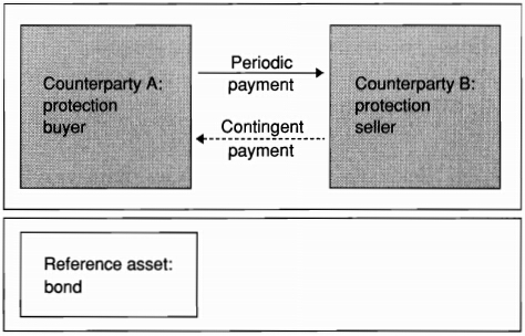
Credit Default Swaps

Definition of CDS

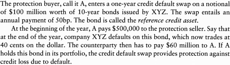
In a credit default swap contract, a protection buyer (say A) pays a premium to the protection seller (say B), in exchange for payment if a credit evet occurs
- the premium payment can be a lump sum or periodic
- the contigent payment is triggered by a credit event (CE) on the underlying credit, say a bond issued by company Y

A CDS is a option instead of a swap
- the main difference from a regular option: the cost of a option is paid in installments instead of up front
- if the cost is paid up front, the contract is called a default put option
- the annual payment is referred as the CDS spread
An example of CDS
Most CDS contracts are quoted in terms of an annual spread, with the payment made on quarterly basis
Default swaps are embedded in many financial products, for example:

Settlement

The payment ( $Q$ ) on default reflects the losses to the holders of the reference asset when the credit event occur. It takes a number of forms:
- cash settlement, or a payment equal to the strike minusthe prevailing market value of the underlying bonds
- physical settlement of the defaulted obligation in exchange for a fixed payment
- a lump sum, or a fixed amount based on some pre-agreed recovery rate. (if the CE occurs, the recovery rate is set at 40%, leading to a payment of 60% of the notional)
The payoff of a CDS is
$\text{Payment}=\text{Notional}\times Q\times I(\text{CE})$
- binary credit default swap: $Q=1$
- with physical settlement, the contract defines a list of bond, which can trade at different prices but must be exchanged for their face value, that can be delivered (delivery option)
- cash settlement can be conducted through an auction, which defines the recovery rate

Pricing

CDS contracts can be priced by considering the present value of the cash flows on each side of the contract.

The value $V$ and the fair spread $s$ of the CDS contract should satisfy the following:

$V=(\text{PV Payoff})-s(\text{PV Spread})=\left(\sum_{t=1}^Tk_t(1-f)PV_t\right)-s\left(\sum_{t=1}^TS_{t-1}PV_t\right)$

The default probabilities used to price the CDS contracts must be risk-neutraal probabilities, not real-world probabilities.

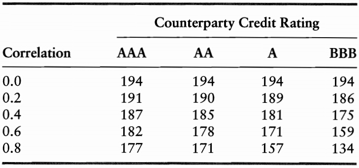
Counterparty Risk

A CDS does not eliminate credit risk entirely.
- the protection buyer decreases exposure to the reference credit Y but assume new credit exposure to the CDS seller
- correlation between the default risk of the underlying credit and of the couterparty is important

A CDS is unfunded
- unfunded: each party is resposible for making payments without recourse to other assets
- ufunded: the protection seller makes a payment that could be used to settle any potential redit event

Other Contracts

CDS Variants

The first-of-basket-to-default swap gives the protection buyer the right to deliver one and only one defaulted security out of a basket of selected securities
- the contract will be more expensive than a single credit swap, all else kept equal
- the price of protection also depends on the correlation between credit events
With an $N$ th-to-default swap, payment is triggered after $N$ defaults in the underlying portfolio, but not before
CDS indices are widely used to track the performance of this market
- the iTraxx indices cover the most liquid names in European and Asian credit markets
- the North American and emerging markets are covered by the CDX indices

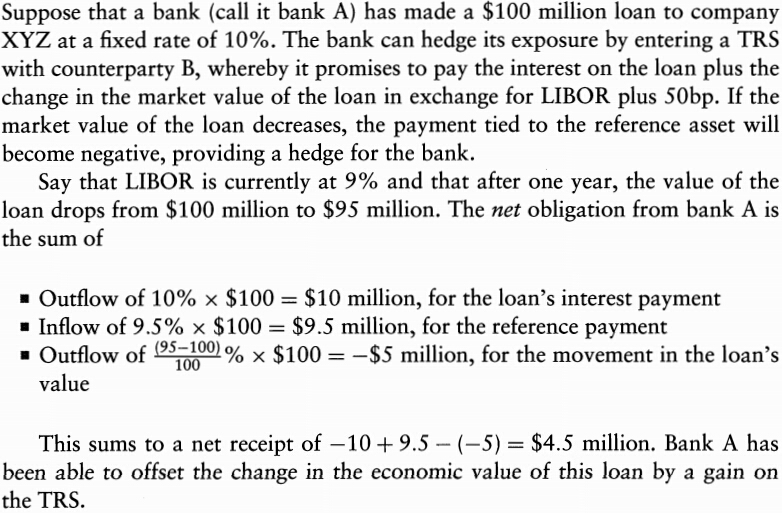
Total Return Swaps

A total return swap (TRS) is a contract where one party, called the protection buyer, makes a series of payments linked to the total return on a reference asset. In exchange, the protection seller makes a series of payments tied to a reference rate, such as the yield on an equivalent Treasury issue (or LIBOR ) plus a spread.

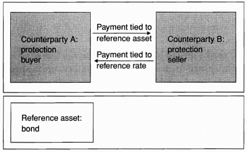
TRS provides protection against credit risk in a mark-to-market (MTM) framework
For the protection buyer, the TRS removes all the economic risk of the underlying asset without selling it
Unlike a CDS, the TRS involves both creditrisk and market risk, the latter reflecting pure interest rate risk

Credit Spread Forwards and Option

In a credit spread forward contract, the buyer receives the difference between the credit spread at maturity and an agreed-upon spread, if positive. Conversely, a payment is made if the difference is negative. The payment is,
$\text{Payment}=(S-F)\times \text{MD}\times\text{Notional}$
Or, equivalently
$\text{Payment}=[P(y+F,\tau)-P(y+S,\tau)]\times\text{Notional}$
In a credit spread option contract, the buyer pays a premium in exchange for the right to put any increase in the spread to the option seller at a predefined maturity:
$\text{Payment}=(S-K)^+\times \text{MD}\times\text{Notional}$

Structured Products

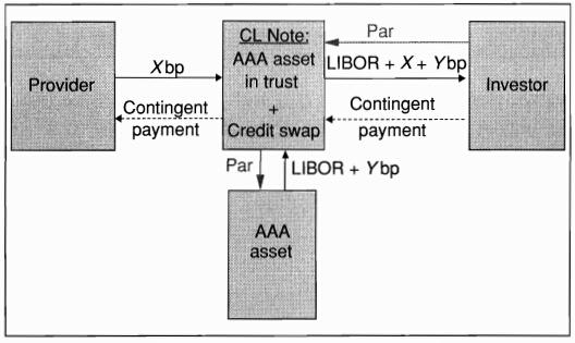
Credit-Linked Notes

Credit-linked notes (CLNs) are structured securities that combine a credit derivative with a regular bond
- the buyer of protection transfers credit risk to an investor via an intermediary bond-issuing entity
- the entity can be the buyer itself or a special-purpose vehicle (SPV)
- this structure may carry a higher yield if the CDS spread is greater than the bond yield spread
- this structure may also be attractive to investors who are precluded from investing directly in derivatives

Collateralized Debt Obligations

The waterfall structure of CDO

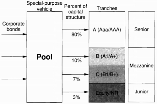
In this example, 80% of the capital structure is apportioned to tranche A, which has the highest credit rating of Aaa, using Moody’s rating, or AAA. It pays LIBOR + 45bp, for example. Other tranches have lower priorities and ratings. These intermediate, mezzanine, tranches are typically rated A, Baa, Ba, or B (A, BBB, BB, B, using S&P's ratings). For instance, tranche C would absorb losses from 3% to 10%. These numbers are called, respectively, the attachment point and the detachment point.

Managing Credit Risk

Measuring the Distribution of Credit Losses

Default mode (DM): considering only losses due to defaults instead of changges in market values

For a portfolio of $N$ conterparties, the credit loss (CL) is
$\text{CL}=\sum_{i=1}^Nb_i\times\text{CE}_i\times\text{LGD}_i$

The net replacement value (NRV)
$\text{NRV}=\sum_{i=1}^N\text{CE}_i$

A typical distribution of credit profits & losses (P&L)
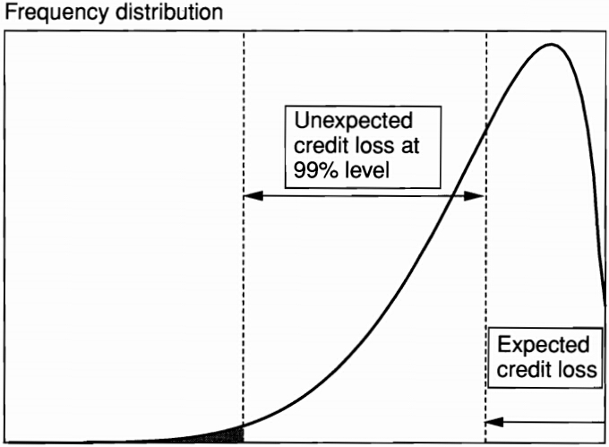
The distribution of P&L is \textit{highly skewed to the left
- similar to a short position in an option
- Merton model:
  $\text{A Risky bond}=\text{A risk-free bond}+\text{short an option}$
Major features
- The Expected credit loss (ECL) represents the average credit loss. The pricing of the portfolio should be such that it covers the expected loss
- The Unexpected credit loss (UCL) represents the loss that will not be exceeded at some level of confidence, typically 99.9%. Taking the deviation from the expected loss gives the unexpected credit loss. The institution should have enough equity capital to cover the unexpected loss.

The effect of correlations

Correlations across default event $b_i$
Correlations across default event and exposure
- wrong-way trades: exposure is positively correlated with the probability of default
- right-way trades occurs when the transaction is a hedge for the counterparty

Measuring Expected Credit Loss

Expected Loss over a Target Horizon

$\begin{array}{lll} &&E[CL]=\int f(b,\text{CE},\text{LGD})(b\times\text{CE}\times\text{LGD})dbd\text{CE}d\text{LGD}\nonumber \end{array}$

Assuming independency,

$\begin{array}{lll} E[CL]&=&\left[\int f(b)(b)db\right]\left[\int f(\text{CE})(\text{CE})d\text{CE}\right]\nonumber\\ &&\left[\int f(\text{LGD})(\text{LGD})d\text{LGD}\right]\nonumber \end{array}$

$\begin{array}{lll} \Longrightarrow \text{ECL}=\Pr(\text{default})\times E[\text{CE}]\times E[\text{LGD}]\nonumber \end{array}$

The Time Profile of Expected Loss

The present value of expected credit losses (PVECL):
$\text{PVECL}=\sum_tE[\text{CL}_t]\times\text{PV}_t=\sum_t[k_t\times\text{ECE}_t\times(1-f)]\times\text{PV}_t$

It can be simplified by adopting the average default probability and average exposure over the life of the asset:
$\text{PVECL}_A=\text{Ave}[k_t]\times \text{Ave}[\text{ECE}_t]\times(1-f)\times\left[\sum_t\text{PV}_t\right]$

An even simpler approach, when ECE is constant, considers the final maturity $T$ only, using the cumulative default rate $c_T$ and discount factor $\text{PV}_T$ :
$\text{PVECL}_F=c_T\times\text{ECE}\times(1-f)\times\text{PV}_T$

Measuring Credit VaR

Credit VaR over a Target Horizon
- At a given confidence level $c$ , the worst credit loss (WCL) is defined such that
  $1-c=\int_{WCL}^{\infty}f(x)dx$
- Credit VaR is defined as the unexpected credit loss at some confidence level, which is measured as the deviation from ECL:
  $\text{Credit VaR}=\text{UCL}=\text{WCL}-\text{ECL}$
- It should be viewed as the economic capital to be held as a buffer against unexpected losses
Using Credit VaR to Manage the Portfolio
- rationales on trades: profitability vs. credit risk (credit VaR)
- the marginal contribution to risk can be used to analyze the incremental effect of a proposed trade on the total portfolio risk
- the marginal analysis can also help to establish the renumeration of capital required to support the position

Portfolio Credit Risk Models

Approaches to Portfolio Credit Risk Models

Model Type
- Top-down models group credit risks using single statistics. They aggregate many sources if risk viewed as homogeneous into an overall portfolio risk, without going into the details of individual transactions. It is appropriate for retail portfolios with large numbers of credits, but less so for corporate or sovereign loans.
- Bottom-up models account for futures of each instrument. It is most similar to the structural decomposition of positions that characterizes market VaR systems. It is appropriate for corporate and capital market portfolios. It is also most useful for taking corrective action, because the risk structure can be reverse-engineered to modify the risk profile
Risk Definitions
- Default-mode models consider only outright default as a credit event
- Mark-to-market (MTM) models consider changes in market values and ratings changes, including defaults
Models of Default Probability
- Conditional models incorporate changing macroeconomic factors into teh default probability through a functional relationship
- Unconditional models have fixed default probabilities and tend to focus on borrower-or factor-specific information
Models of Default Correlations
- Structural Models explain correlations by the joint movements of assets
- Reduced-form models explain correlations by assuming a particular functional relationship between the default probability and background factors
Comparison of Credit Risk Models