L03 Volatility and Mortgage-Backed Securities Risk

• L03 Volatility and Mortgage-Backed Securities Risk
  • Managing Volatility Risk
    • Historical Volatility & Historical Correlation
      • Volatility
      • Historical Vol Forecasts
      • Some illustrative H vols
      • EWMA
      • EWMA Forecasting
      • GARCH models
      • GARCH$(1,1)$
      • Properties of GARCH
      • Forecasting with GARCH
      • Estimating GARCH models
      • Other GARCH models
      • Covariances and correlations
    • Implied Volatility & Implied Correlation
      • Implied Volatility
      • VIX
      • Implied Volatility Surface
      • Prediction of the Volatility Surface
      • Implied Correlation
      • Currency Implied Correlation: A Triplet of Currency Options
      • Portfolio Average Correlation
    • Covariance Matrices
      • Forecasting covariance matrices
      • Generating PD or PSD covariance matrices
      • Computational problems
    • Variance Swaps
      • Variance Swaps
    • Dynamic Trading
      • Dynamic Optoin Replication
      • Static Optoin Replication
      • Implications for Trading
  • Mortgage-Backed Securities Risk
    • Prepayment Risk
      • Mortgage as Annuities
      • Prepayment Speed
      • Measuring Prepayment Risk}
    • Securitization
      • Priciples of Securitization
      • Issues with Securitization
      • Rethinking Securitization
    • Tranching
      • Concept
      • Inverse Floaters
      • CMOs

Managing Volatility Risk

Historical Volatility & Historical Correlation

Volatility

• Can define as std of returns

• Helpful to standardise on an annualised basis

• If volatility is constant, we can derive longer-period volatility from (in)famous 'square-root rule'
  $$\sigma|_{h-\text{period}}=\sqrt{h}\sigma|_{1-\text{period}}$$

• Important for derivatives pricing, hedging, and risk measurement

---

Historical Vol Forecasts

• One forecasting rule is the historical MA
  $$\sigma_t^2=\frac{1}{n-1}\sum_{i=1}^n(x_{t-i}-\bar{x}_t)^2$$

• This gives unbiased estimate

• If data period is daily, mean return will be low and we can set this to zero
  $$\sigma_t^2=\frac{1}{n}\sum_{i=1}^nx_{t-i}^2$$

• This usually reduces variance

• Change from $n-1$ to n in denominator makes little difference

• These approaches give each observation the same weight, then no weight, in forecast

• Easy to use

• Problems

  • If true vol is constant, any differences are due only to sampling error
  • Can’t allow for changes in true vol
  • More distant events in sample period have same weight as more recent ones

---

Some illustrative H vols

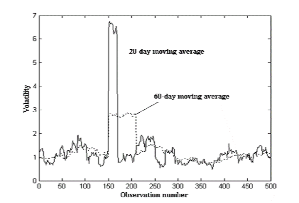
• Figure gives two alternative H estimators, using $n=20$ and $n=60$
• For large $n$, vol estimate is smoother and less responsive
• When shock occurs, both jump and remain high
• For high $n$, plateau is lower but longer lasting

---

EWMA

• Can ameliorate some of these problems using an exponential weight

• Weight attached to observation decays over time
  $$\sigma_t^2\approxeq(1-\lambda)\sum_{i=1}^n\lambda^{i-1}x^2_{t-i}$$

• Can also be rewritten as updating rule
  $$\sigma_t^2=\lambda\sigma^2_{t-1}+(1-\lambda)x^2_{t-1}-(1-\lambda)\lambda^nx^2_{t-n-1}\approxeq\lambda\sigma^2_{t-1}+(1-\lambda)x_{t-1}^2$$

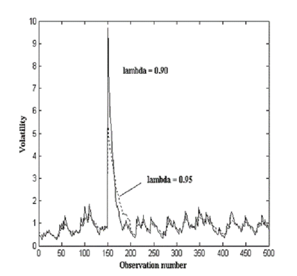
• Higher $\lambda$ means weight declines slowly
• For daily data, RiskMetrics uses $\lambda=0.94$
• Figure shows how low- $\lambda$ rises most after shock, but decays faster

---

EWMA Forecasting

• Can use EWMA to forecast:
  $$E[\sigma^2_{t+k}]=\sigma^2_t$$
  for any $k>0$

• EWMA forecast is same as current value

• But flat vol forecast not very appealing

  • Ignores other information; not plausible

---

GARCH models

• EWMA models also take $\lambda$ to be constant

• This is implausible and not appealing

• Popular alternative is a GARCH

• This fits nicely with some stylised features of returns

  • Returns show vol clustering
  • Returns show leptokurtosis – heavy tails

• GARCH can accommodate both of these

• Basic GARCH$(p,q)$ model
  $$\sigma_t^2=\omega+\alpha_1\epsilon_{t-1}^2+\dots+\alpha_p\epsilon_{t-p}^2+\beta_1\sigma_{t-1}^2+\dots+\beta_q\sigma_{t-q}^2$$
  for $\omega>0$ and $\alpha_i,\beta_j>0,\ \forall i,j$

• Errors are often normal, in which case return are conditionally normal

• Returns can be $t$ also

---

GARCH$(1,1)$

• Most popular is GARCH$(1,1)$
  $$\sigma^2_t=\omega+\alpha x^2_{t-1}+\beta\sigma_{t-1}^2$$
  $$\omega>0\text{; }\alpha,\beta>0\text{; }\alpha+\beta<1$$

• High $\beta$ implies that vol is persistent and takes a long time to change

• High $\alpha$ means that vol is spikey and quick to react

• Often $\beta$ is over 0.7 and $\alpha$ less than 0.25

---

Properties of GARCH

• GARCH$(1,1)$ depends on same variables as EWMA, but has three parameters not 1

• EWMA is special case with $\omega=0$, $\alpha=1-\lambda$ and $\beta=\lambda$

• GARCH$(1,1)$ with positive intercept $\omega$ allows vol to be mean-reverting

  • This is appealing
  • Long run vol tends to revert to $\omega/(1-\alpha-\beta)$

---

Forecasting with GARCH

• Letting $V=\omega/(1-\alpha-\beta)$, can show that $k-$period ahead forecast is
  $$E[\sigma^2_{t+k}]=V+(\alpha+\beta)^k(\sigma^2_t-V)$$

• Since $\alpha+\beta<1$, this means vol forecast converges to $V$

• Can also apply to vol term structure

---

Estimating GARCH models

• Run data through a preliminary filter (e.g., ARMA) to remove serial correlation

• ARMA model should be as parsimonious as possible

• Select particular candidate GARCH specification (e.g., based on PACs)

• Estimate model using ML

• Check model adequacy by testing whether standardised innovations are idd and follow assumed distribution

• Pass or fail model

• If model fails, try another GARCH

---

Other GARCH models

• IGARCH is applicable when returns not stationary
  $$\sigma^2_t=\omega+\beta\sigma^2_{t-1}+(1-\beta)x^2_{t-1}$$

  • EWMA is special case where $\omega=0$

• Components GARCH

  • Lets vol converge to a long-term vol that changes over time

• Factor GARCH

  • This links returns from n assets to one or more underlying factors (e.g., as with CAPM)
    $$r_{it}=\alpha_i+\beta_iM_i+\epsilon_{it}$$
  • This leads to
    $$\sigma^2_{it}=\beta^2\sigma_{Mt}^2+\sigma_{\epsilon_{it}}^2$$

---

Covariances and correlations

• Covarance between $X$ and $Y$ is
  $$\sigma^2_{XY}=E[XY]-E[X]E[Y]$$

• Correlation is
  $$\rho_{XY}=\frac{\sigma^2_{XY}}{\sigma_{X}\sigma_{Y}}$$

• Correlation only good measure of dependency is returns are elliptical
  Only defined if vols exist – need to check for this

• Estimate correlation

  • Equal-weighted covariance/correlation
  • EWMA covariances/correlation
  • GARCH covariances/correlation

---

Implied Volatility & Implied Correlation

Implied Volatility

• Black-Scholes model
  $$c=S_0N(d_1)-Ke^{-r\tau}N(d_2)$$
  $$p=Ke^{-r\tau}N(-d_2)-S_0N(d_1)$$
  where
  $$d_1=\frac{\ln(S_0/K)+(r+\sigma^2/2)\tau}{\sigma\sqrt{\tau}}$$
  $$d_2=\frac{\ln(S_0/K)+(r-\sigma^2/2)\tau}{\sigma\sqrt{\tau}}=d_1-\sigma\sqrt{\tau}$$

• Implied volatility $ISD_t=f^{-1}(c_t,S_t,r_t,K,\tau)$

• Quote ISD vs premium

  • ISD is more intuitive (similar to quotting bonds with yield instead of price)
  • reflect the market's view
  • ISD is a risk-neutral volatility

• These are volatilities generated from option prices

• Given that other variables (price, etc.) are observable, can infer implied vol from option price (e.g., Black-Scholes)

• Implied vol is a forward-looking estimator

  • Takes account of all information, not just historical backward-looking information

• Implied vols generally regarded as better than historical ones

• mplied vols are dependent on option-pricing model

  • Possible problems due to holes in Black-Scholes, volatility smiles/smirks, etc.

• Also, implied vols only exist for assets on which options have been written

---

VIX

• VIX is a popular measure of the implied volatility of S&P 500 index options
  
  
  
  
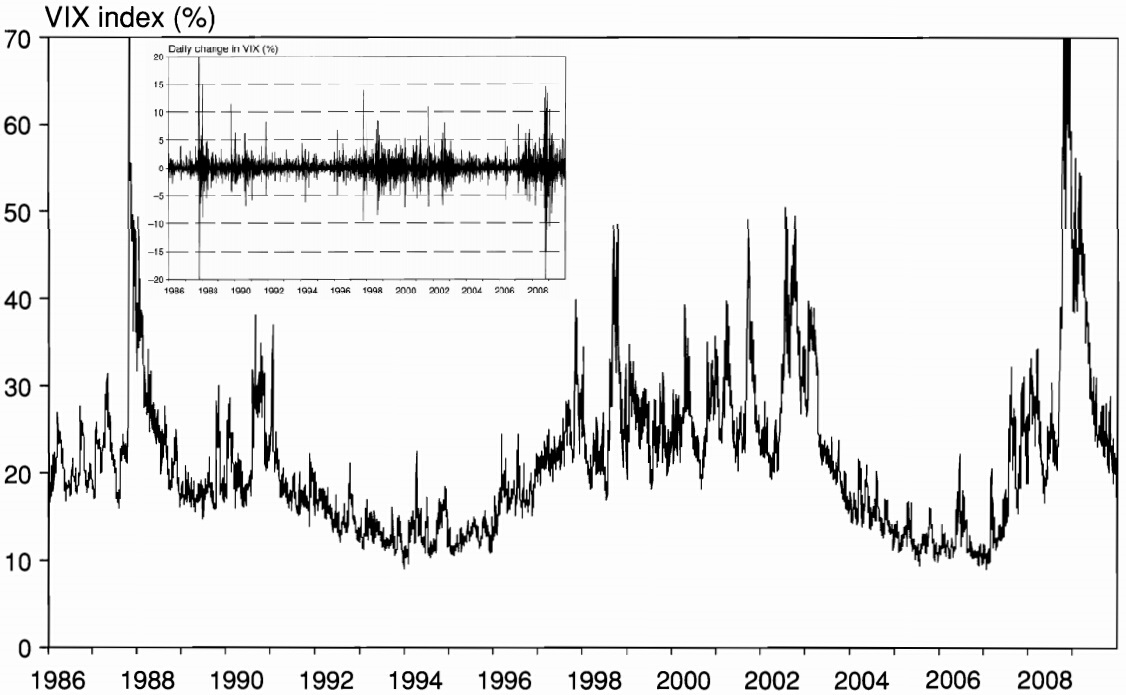
• Properties about VIX
  • average value: on the order of 21%; daily change: about 2.4%
  • assuming normal distribution: daily movements should be within $\pm5\%$
  • the actual distribution is far from normal

---

Implied Volatility Surface

• If B-S were correct, the ISDs should be constant across strike prices and maturities

• If we plot ISDs agaist strike prices and maturities we obtain the implied volatility surface
  
  
  
  

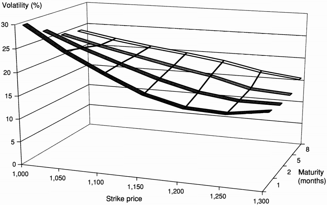
  • volatility smile (ISDs vs. strike prices)
  • term structure of volatility
  • spot & forward volatility $\sigma_2^2\times\tau_2=\sigma^2_1\times\tau_1+\sigma^2_{1,2}\times(\tau_2-\tau_1)$

---

Prediction of the Volatility Surface

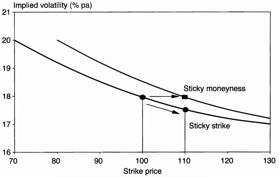
• Sticky strike

  • there is no structural change in the volatility curve
  • peice movement is largely temporary

• Sticky moneyness

  • permanent shift in the volatility curve

---

Implied Correlation

• These are directly analogous to implied volatilities

• But can only use if relevant options exist

• Need two or more options, or spread options

• Have same pros and cons as implied vols, and also be unstable

• Exchange option involves the surrender of an asset (B) in exchange for acquiring another (A). The payoff on such a call is
  $$c_T=\max(S^A_T-S_T^B,0)$$

• The valuation formula (**Margrabe Model})

  • replace $K$ by the price of asset B ($S_B$)
  • replace the risk-free rate by the yield on asset B ($q_B$)
  • the volatility is $\sigma_{AB}^2=\sigma_A^2+\sigma_B^2-2\rho\sigma_A\sigma_B$

• Rainbow Option: exposed to two or more sources of uncertainty

  • e.g. An option on a basket

---

Currency Implied Correlation: A Triplet of Currency Options

• Exchange rates are expressed relative to a base currency (usually USD)

• The cross rate is the exchange rate between two currencies other than the reference currency

• Example: let $S_1$ be the dollar price of GBP and $S_2$ be the doller/euro rate. Then the euro/pound rate is
  $$S_3(\text{EUR/GBP})=\frac{S_1(\text{\$/GBP})}{S_2(\text{\$/EUR})}$$
  $$\Longrightarrow\ln[S_3]=\ln[S_1]-\ln[S_2]$$
  the volatility of the cross rate is
  $$\sigma_3^2=\sigma_1^2+\sigma_2^2-\rho_{12}\sigma_1\sigma_2$$

---

Portfolio Average Correlation

• Expressing portfolio ISD by the ISD of its components through the average correlation
  $$\begin{array}{lll} \sigma_p^2&=&\sum_{i=1}^N\omega_i^2\sigma_i^2+2\sum_{i=1}^N\sum_{j<i}^N\omega_i\omega_j\rho_{ij}\sigma_i\sigma_j\\ &=&\sum_{i=1}^N\omega_i^2\sigma_i^2+2\sum_{i=1}^N\sum_{j<i}^N\omega_i\omega_j(\rho)\sigma_i\sigma_j \end{array}$$

  • the average correlation $\rho$ is a summary measure of diversification benefits across the portfolio
  • all else equal, an increasing correlation in creases the total portfolio risk

• A dispersion trade takes a short position in index volatility, which is offset by long position in the volatility of the index components

---

Covariance Matrices

Forecasting covariance matrices

• Estimated cov or corr matrices must be positive definite or positive semi-definite

  • This imposes constraints on how we can estimate them
  • Can’t estimate parameters independently, and then hope for this condition to be satisfied

• Historical covariance matrices

  • Straightforward to estimate:

    • Choose window size, and estimate parameters simultaneously

  • Drawbacks

    • Only accurate if true matrix constant
    • Can suffers from ghost effects

• Multivariate EWMA

  • This is more flexible and has smaller ghost effects
  • Must choose same decay factor for all terms
  • If we don’t, there is no guarantee that matrix will be PD or PSD

• Multivariate GARCH

  • This can be difficult

    • Can need a lot of parameters
    • High dimensions hard to handle
    • Problems of convergence of routines, etc.

  • Can use methods such as orthogonal GARCH to get around some of these problems

---

Generating PD or PSD covariance matrices

• One way to ensure PD or PSD matrices is to adjust eigenvalues, and then recover matrix from adjusted eigenvalues

  • If we want PD, eigenvalues must be positive
  • If we want PSD, eigenvalues must be non-negative

• Obtain eigenvalues, adjust any –ve (and maybe 0) ones using some rule

• Adjusted matrix satisfies our requirements

---

Computational problems

• Even if true matrix is PD (or PSD), estimated matrix might not be

• Risk factors might be highly correlated

• This can produce 0 or –ve estimated eigenvalues

• These problems can be aggravated if covariance matrix is used for trading or risk management

• Possible answers:

  • Choose risk factors that are not too highly correlated
  • Don't choose too many risk factors
  • Alternatively, can adjust eigenvalues

---

Variance Swaps

Variance Swaps

• A variance swap is a forward contract on the realized variance, the payoff is
  $$V_T=(\sigma_{t_0,T}^2-K_V)N,\text{ }\sigma^2=\frac{252}{\tau}\sum_{i=1}^\tau[\ln(S_i/S_{i-1})]^2$$

  • it can be written on any asset (usually equities or equity indices)
  • A correlation swap is similar to a variance swap, however its payoff is tied to the realized average correlation in a portfolio over the selected period

• e.g. A one yield contract on S&P 500 index: $K_V=(15\%)^2$, $N=\$100,000/(\text{one volatility point})$. If $\sigma=17\%$, the payoff to the long position is
  $$[\$100,000/(1)^2]\times[17^2-15^2]=\$6,400,000$$

• Market value of an variance swap
  $$V_t=Ne^{-r\tau}[\omega(\sigma^2_{t_0,T}-K_V)+(1-\omega)(K_t-K_V)]$$

• Correlation trading

---

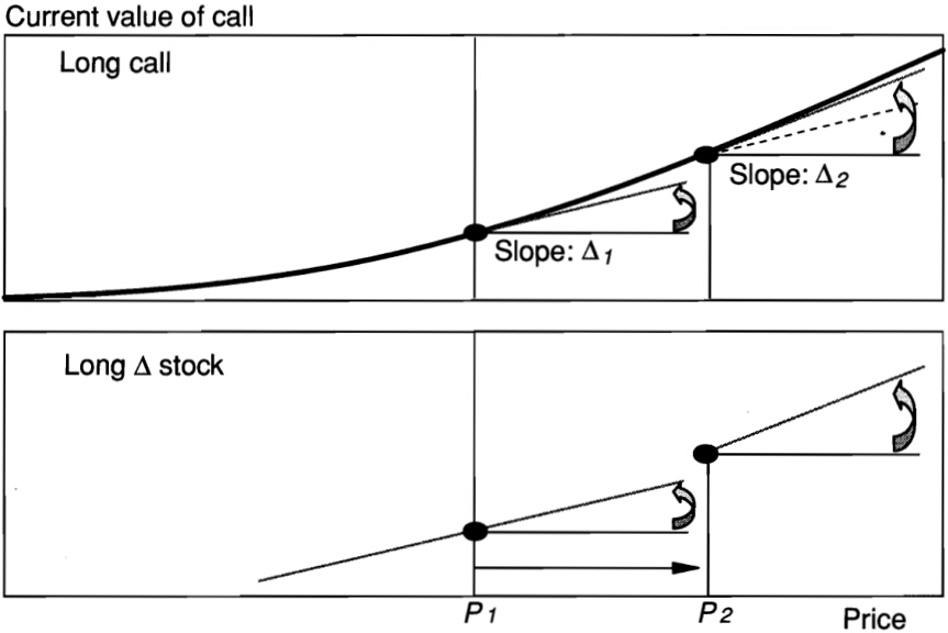
Dynamic Trading

Dynamic Optoin Replication

Holding a call option is equivalent to holding a fraction of underlying asset

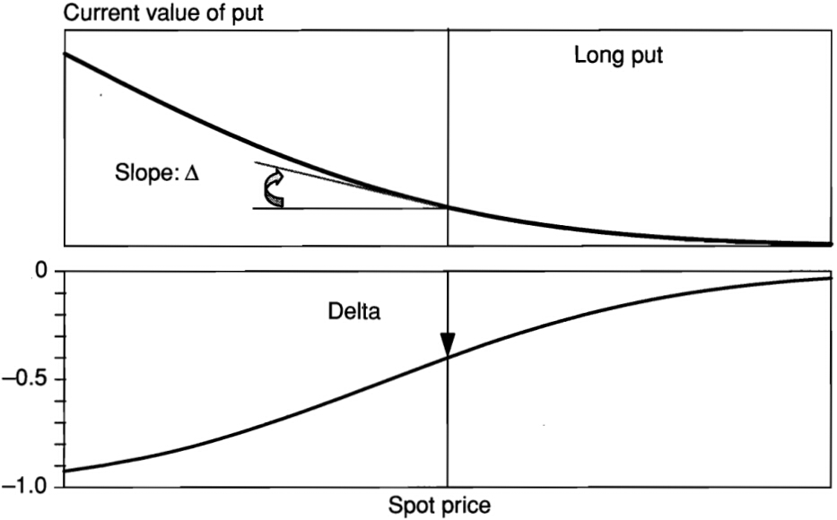
Dynamic replication of a put

---

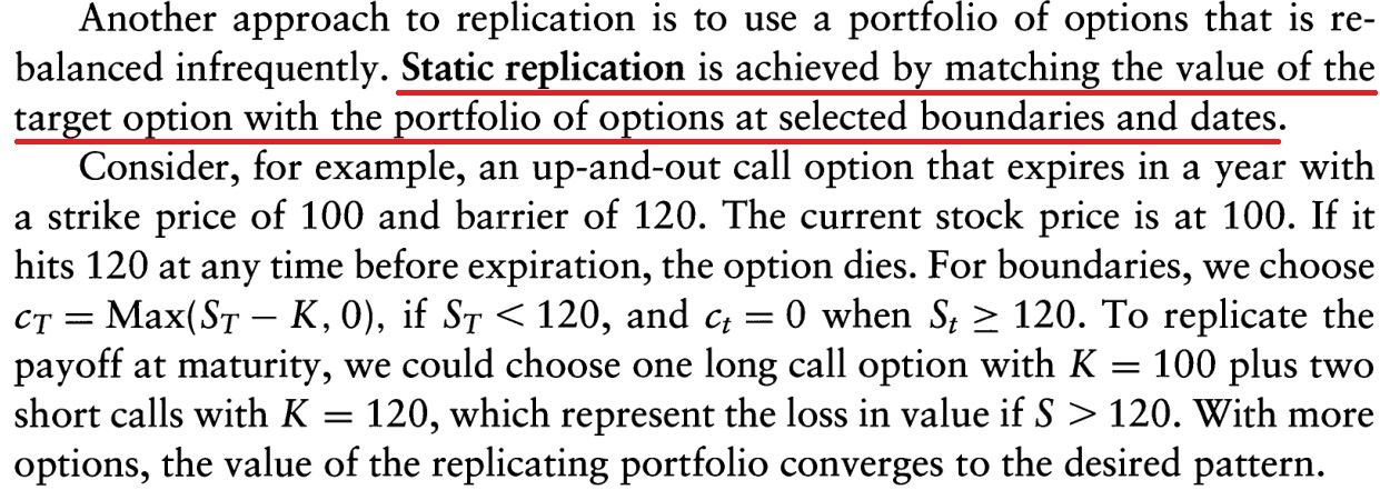
Static Optoin Replication

---

Implications for Trading

• Dynamic replication of a long option is bound to loss money

  • it buys the asset *after} the price has gong up (too late)
  • the loss of each transaction will culmulate to an option premium, which is driven by the realized valotility

• Selling an option and dynamically hedging it using the underlying instrument

  • the strategy is delta-neutral
  • revenue from selling an option: a function of implied volatility
  • cost from dynamic hedging: a function of realized volatility
  • in equity markets, implied volatility tends to be greater than the realized volatility

• More general implications

  • large scale automatic trading system have the potential to be destabilizing
  • selling an asset after its price has gong down is similar to prudent risk-management practices

---

Mortgage-Backed Securities Risk

Prepayment Risk

Mortgage as Annuities

• Mortgages can be structured to have fixed or floating payments. Assuming a fixed monthly payment $C_t$,the price-yield relationship is $P=\sum_{t=1}^T\frac{C_t}{(1+y)^t}$
  
  
  
  

• Life of bond

  • maturity
  • average life (AL): $AL=\sum_{t=1}^Tt\color{red}{P_t/P}$
  • duration: $D=\sum_{t=1}^Tt\color{red}{C_t(1+y)^{-t}/P}$

• When dealing with pool of mortgages, we use

  • weighted average maturity (WAM)
  • weighted average maturity coupon (WAC)
  • weighted average maturity life (WAL)

---

Prepayment Speed

• Factors which affect mortgage refinancing patterns / prepayment speed

  • spread between the mortgage rate and current rates
  • age of the loan
  • refinancing incentives
  • previous path of interest rates
  • level of mortgage rate
  • economic activity
  • seasonal effects

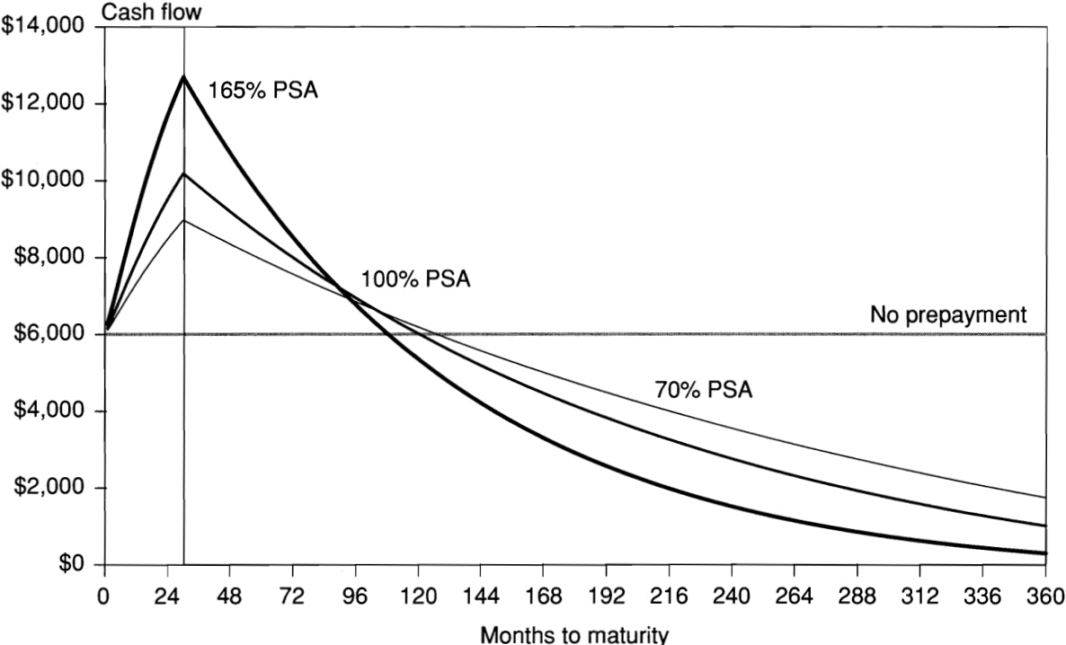
• Conditional prepayment rate (CPR) & single month mortality (SMM)
  
  
  
  

Public Securities Association (PSA) Prepayment Model:
$$CPR=\min[6\%\times(t/30),6\%]$$
By converntion, prepayment patterns are expressed as a percentage of the PSA speed.

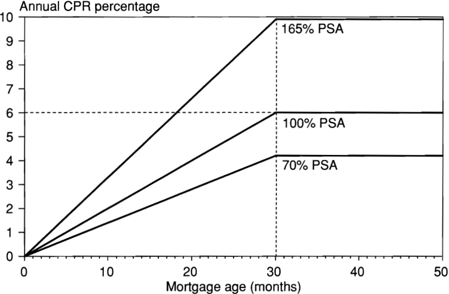
Project cash flows based on the prepayment speed pattern.

---

Measuring Prepayment Risk}

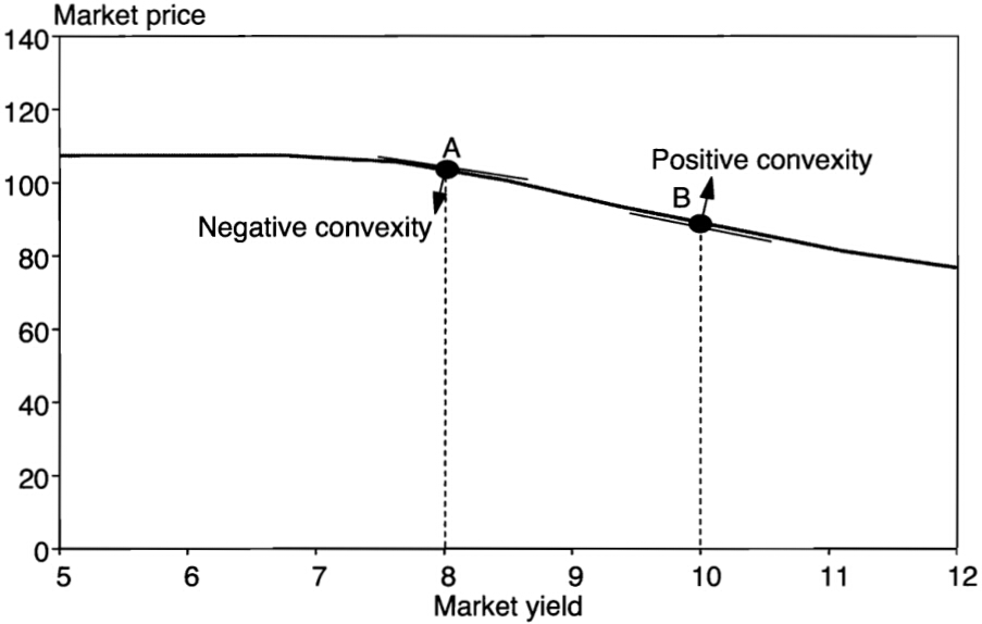
• Prepayment risk

  • contraction risk: low rate $\rightarrow$ more prepayment $\rightarrow$ shorter average life
  • extension risk: high rate $\rightarrow$ less prepayment $\rightarrow$ longer average life

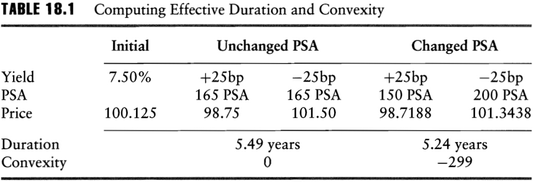
• Dealing with the changing cash-flow pattern

  • effective duration
    $$D^E=\frac{P(y_0-\Delta y)-P(y_0+\Delta y)}{2P_0\Delta y}$$
  • effective convexity
    $$C^E=\left[\frac{P(y_0-\Delta y)-P_0}{P_0\Delta y}-\frac{P_0-P(y_0+\Delta y)}{P_0\Delta y}\right]\bigg/\Delta y$$

• The option component

  • prepayment represents a long position in option for the borrower
  • prepayment represents a short position in option for the lender

• Option-Adjusted Spread (OAS)

  • static spread (SS): the difference between the yield of the MBS and that of a Treasury note with the same weighted average life
  • zero spread (ZS): a fixed spread added to zero-coupon rate so that the discounted value of the projected cash flows equals the current price
    $$P=\sum_{t=1}^T\frac{C_t}{(1+R_t+ZS)^t}$$
  • The OAS method involves running simulations of various scenarios and prepayments to establish the option cost
    $$\text{OAS}=\text{Zero Spread}-\text{Option Cost}$$

---

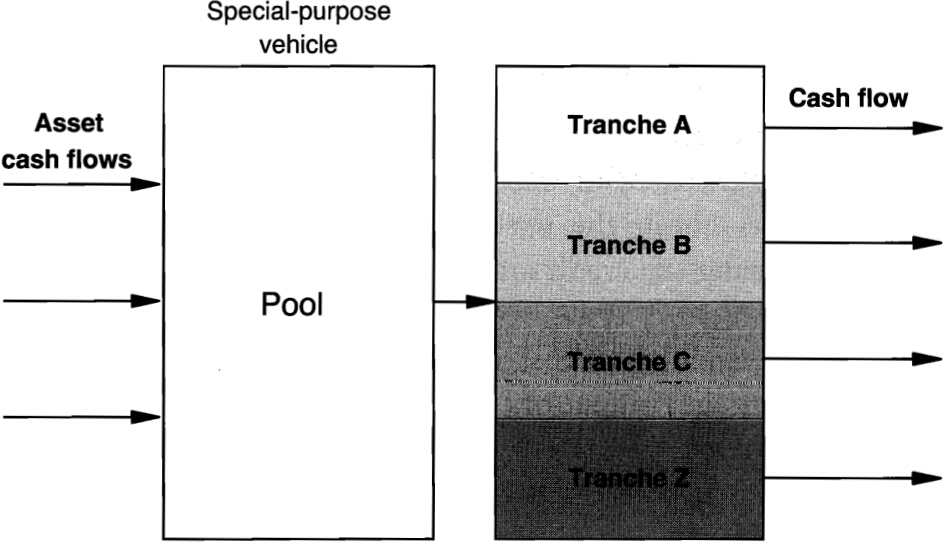
Securitization

Priciples of Securitization

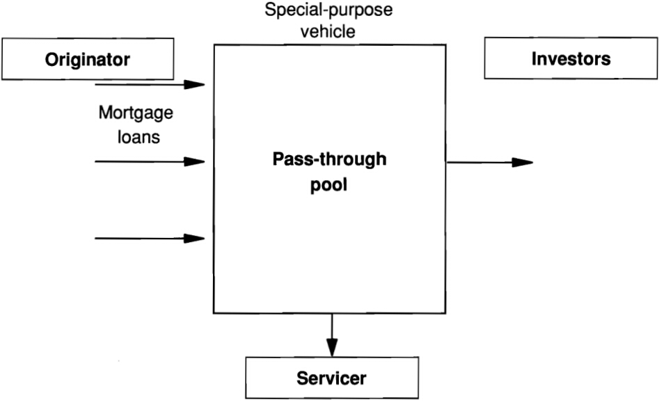
• Procedures of securitization (off-balance-sheet)

  • create a special purpose vehicle (SPV), or special-purpose entity (SPE)
  • the originator pools a group of assets and sells them to the SPV
  • SPV issues tradable claims, or securities, that are backed by the financial assets

• Advantage of this structure

  • it shields the asset-backed security (ABS) investor from the credit risk of the originator
  • pooling offers ready-made diversification across many assets

• All sorts of assets (collateral) can be included in ABSs

  • mortgage loans, student loans, credit card receivables, account receivables, debt obligations, and etc.
  • RMBSs: backed by residential mortgage loan
  • CMBSs: backed by commercial mortgage loan
  • the cash flow of RMBSs and CMBSs is subject to interest rate risk, prepayment risk, and default risk

• Structure of securitization

  • pass-through: the SPV issues single class of security
  • tranching: the SPV issues different classes of securities

• On-balance-sheet securitizations (covered bonds or Pfandbriede in Germany)

  • banks originates the loans and issues securities secured by these loans, which are kept on its books
  • investors have recourse against the bank in the case of defaults on the motgage
  • banks provides a guarantee against credit risk

---

Issues with Securitization

• The moral hazard problem

• The adverse selection problem

• cerdit rating fails for securitization that with complex structures

• Securitization pushes housing prices away from their fundamental values

• When the securitization markets froze, many banks and loan originators were stuck with loans that were warehoused, or held in a pipeline that was supposed to be temporary

---

Rethinking Securitization

Tranching

Concept

• Cash flows are redistributed to fit investors' need

  • however, cash flows and risks are fully preserved
  • they are only redistributed across tranches
  • weighted duration & convexity of the portfolio of tranches must add up to the original duration and convexity

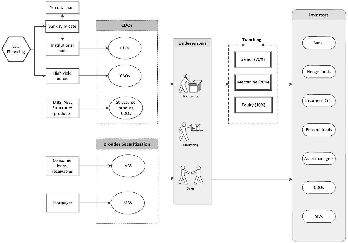
• This structure applies to collateralized mortgage obligations (CMOs), collateralized bond obligations (CBOs) collateralized loan obligations (CLOs), collateralized debt obligations (CDOs)

---

Inverse Floaters

$$\text{Coupon}_F=\min(\text{LIBOR},12\%),\text{ }\text{Coupon}_F=\max(12\%-\text{LIBOR},0)$$

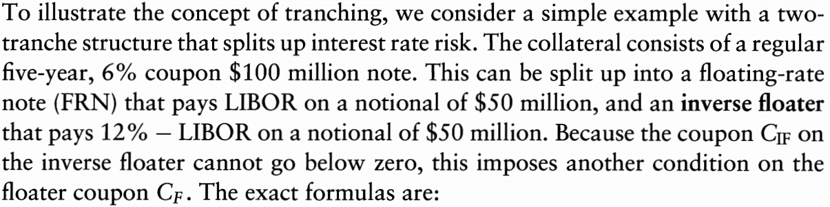
• Try to verify that the outgoing cash flows exactly add up to the incoming cash flows
• Suppose the dollar duration of the original five-year note is 4.5 years, try to analyze the duration of the floater and the inverse floater just before a reset
• What if the coupon is tied to twice LIBOR, i.e. $18\%-2\times\text{LIBOR}$?

---

CMOs

• Sequential-pay tranches: defined by prioritizing the payment of principal into different tranches

• Planned amortization class (PAC)

  • PAC bonds offer a fixed redemption schedule as long as prepayments on the collateral stays within a specified PSA range (say 100 to 250 PSA), called the **PSA collar}
  • the principal payment is set at the minimum payment of these two extreme values for every month of its life
  • all prepayment risk is transfered to other bonds in the CMO structure, called **support bonds}.

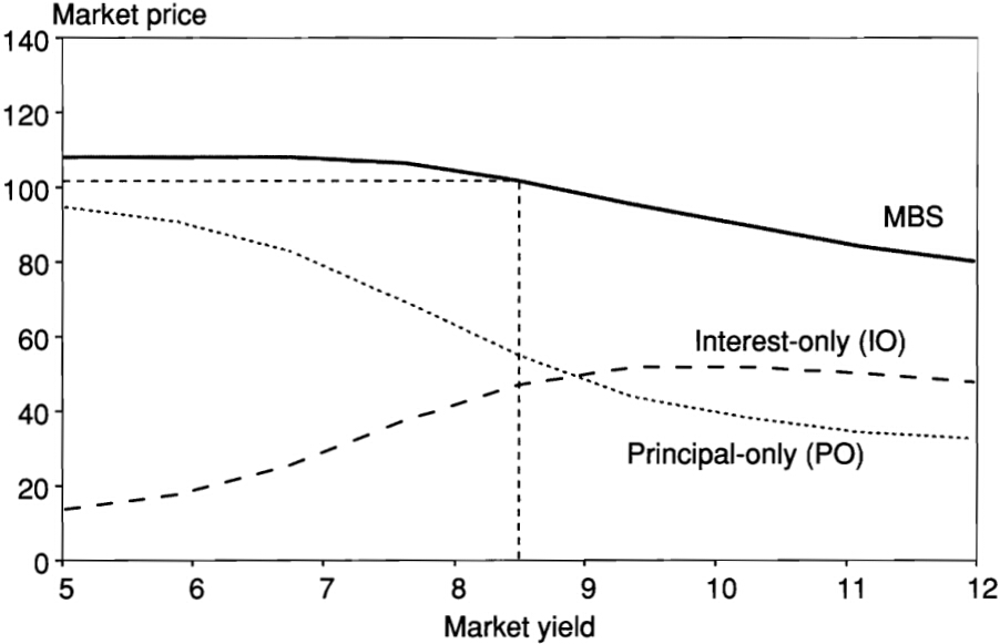
• IO/PO structure: strips the MBS into two components

  • the **interest-only (IO)} tranche receives only the interest payments on the underlying MBS
  • the **principal-only (PO)} tranche receives only the principal payments on the underlying MBS
  • interest rate fall $\rightarrow$ principal payments come early $\rightarrow$ PO appreciate in value while IO depreciate in value