L02 Risk Models & Market Risk

L02 Risk Models & Market Risk

Financial Risk Management Fundamental

Financial Risk

Definition

Financial risk: prospect of financial gain or loss due to unforeseen changes in risk factors
Market risks: arising from changes in market prices or rates
Interest-rate risks, equity risks, exchange rate risks, commodity price risks, etc.
Market vs. credit vs. operational risks
- Credit risks: risks arising from possible default on contract
- Op risks: risks from failure of people or systems

Contributory factors: volatile environment

Stock market volatility
- 23% fall in Dow Jones on Oct. 19, 1987
- Dow Jones fell around 20% in July-Aug 1998
- Massive falls in East Asian stock markets in 1998
- 2015–16 Chinese stock market turbulence
Exchange rate volatility
- Problems of ERM (Exchange Rate Mechanism), peso, rouble, East Asia, etc.
Interest rate volatility
- US interest rates doubled over 1994
Commodity market volatility
- Electricity prices, etc.

Contributory factors: growth in trading activity

Number of shares traded on NYSE grown from 3.5m in 1970 to 100m in 2000
Turnover in FX markets grown from $1bn a day in 1965 to $1,210bn in April 2001
Explosion in new financial instruments
Securitization
Growth of offshore trading
Growth of hedge funds
Derivatives
- Few derivatives until early 1970s
- FX futures (CME, 1972), equity calls (CBOT, 1973), interest-rate futures (1975)
- Swaps and exotics (1980s)
- Cat, credit, electricity, weather derivatives (1990s)
- Daily notional principals negligible in early 1970s; up to nearly $2,800bn in April 2001

Contributory factors: advances in IT

Huge increases in computational power and speed
- Costs falling at 25-30% a year for 30 years
Improvements in software
Improvements in user-friendliness
- E.g., in simulation software
Risk measurers no longer constrained to simple back-of-the-envelope methods

Financial Risk Management before VaR

Risk measurement before VaR

Gap analysis
PV01 analysis
Duration and duration-convexity analysis
Scenario analysis
Portfolio theory
Derivatives risk measures
Statistical methods, ALM, etc.

Gap Analysis

Developed to get crude idea of interest-rate risk exposure
Choose horizon, e.g., 1 year
Determine how much of asset or liability portfolio re-prices in that period
- Rate-sensitive assets / liabilities
GAP = RS assets – RS liabilities
Exposure is change in change in net interest income when interest rates change
- $\Delta\text{NII}=\text{GAP}\times\Delta r$
Pros
- Easy to carry out
- Intuitive
Cons
- Crude
- Only applies to on-balance sheet IR risk
- Looks at impact on income, not asset / liability values
- Results sensitive to choice of horizon

PV01 Analysis

Also applies to fixed income positions
Addresses what will happen to bond price if interest rises by 1 basis point
Price bond at current interest rates
Price bond assuming rate rise by 1 bp
Calculate loss as current minus prospective bond prices

Duration Analysis

Another traditional approach to IR risk assessment
Duration $D$ is weighted average of maturities of a bond’s cashflows,
- weights are present values of each cashflow, divided by PV of all cashflows
- $D=\frac{\sum_tt\times\text{PVCF}_t}{\sum_t\text{PVCF}_t}=\sum_tt\times\color{red}{\frac{\text{PVCF}_t}{\sum_t\text{PVCF}_t}}$
Duration indicates sensitivity of bond price to change in yield:
- $\frac{\Delta P}{\Delta y}=-PD\Longleftrightarrow\frac{\Delta P}{P}=-D\Delta y$
Can approximate duration using simple algorithm as $(P_--P_+)/(2P_\Delta y)$ , where $P_0$ is current price, $P_-$ is price when $\Delta y<0$ , $P_+$ is price when $\Delta y>0$
Duration is a linear function: duration of porfolio is sum of durations of bonds in portfolio
Duration assumes $P-y$ relationship is linear when it is typically convex
Duration ignores embedded options
Duration analysis supposes that yield curve shifts in parallel

Convexity

\small

If duration takes a $P-y$ relationship as linear, convexity takes it as (approx) quadratic
Convexity is the second order term in a Taylor series approximation
$\Delta P/P\approxeq-D\Delta y+(1/2)C(\Delta y)^2$
Convexity is defined as $C=(\Delta^2P/\Delta y^2)/P$
Convexity term gives a refinement to the basic duration approximation
In practice, convexity adjustment often small
Convexity a valuable property
Makes losses smaller, gains bigger
Can approximate convexity as
$C\approxeq(P_-+P_+-2P_0)/(P_0\Delta y^2)$

Pros and cons of duration-convexity

Pros
- Easy to calculate
- Intuitive
- Looks at values, not income
Cons
- Crude (only first-order approx, problems with non-parallel moves in spot rate curve, etc.)
- Often inaccurate even with refinements (e.g., convexity)
- Applies only to IR risks

Scenario Analysis

'What if' analysis – set out scenarios and work out what we gain/lose
Select a set of scenarios, postulate cashflows under each scenario, use results to come to a view about exposure
SA not easy to carry out
- Much hinges on good choice of scenario
- Need to ensure that scenarios do not involve contradictory or implausible assumptions
- Need to think about interrelationships involved
- Want to ensure that all important scenarios covered
SA tells us nothing about probabilities
- Need to use judgement to determine significance of results
SA very subjective
Much depends on skill and intuition of analyst

Portfolio Theory

Starts from premise that investors choose between expected return and risk
- Risk measured by std of portfolio return
Wants high expected return and low risk
Investor chooses portfolio based on strength of preferences for expected return and risk
- Investor determines efficient portfolios, and chooses the one that best fits preferences
Investor who is highly (slightly) risk averse will choose safe (risky) portfolio
Key insight is that risk of any position is not its std, but the extent to which it contributes to portfolio std
- Asset might have a high std, but contribute small risk, and vice versa
Risk is measured by beta (\alert{why?}) – which depends on correlation of asset return with portfolio return
High beta implies high correlation and high risk
Low beta implies low correlation and low risk
Zero beta implies no risk
Ideally, looking for positions with negative beta
- These reduce portfolio risk
PT widely used by portfolio managers
But runs into implementation problems
- Estimation of beta highly problematic
- Each beta is specific to data and portfolio
- Need a long data set to get reliable result
Practitioners often try to avoid some of these problems by working with `the' beta (as in CAPM)
- But this often requires CAPM assumptions to hold
- One market risk factor, etc.
CAPM discredited (Fama-French, etc.)

Derivatives risk measures

Can measure risks of derivatives positions by their Greeks
- Delta $\Delta$ gives change in derivatives price for small change in underlying price
- Gamma $\Gamma$ gives change in derivatives delta for small change in underlying price
- Rho $\rho$ gives change in derivatives price for small change in interest rate
- Theta $\Theta$ gives change in derivatives price for small change in time to maturity
- Vega $\nu$ (\alert{which is not really a Greek letter}) gives change in derivatives price for small change in volatilty
Use of Greeks requires considerable skill
Need to handle different signals at the same time
Risks measures only incremental
- Work against small changes in exogenous factors
- Can be Greek-hedged, but still be very exposed if there are large exogenous shifts
- Hedging strategies require liquid markets, and can fail if market liquidity dries up (as in Oct 1987)
Risk measures are dynamic
- Can change considerably over time
- E.g., gamma of ATM option goes to infinity

Value at Risk (VaR)

Value at Risk

In late 1970s and 1980s, major financial institutions started work on internal models to measure and aggregate risks across institution
As firms became more complex, it was becoming more difficult but also more important to get a view of firmwide risks
Firms lacked the methodology to do so
- Can't simply aggregate risks from sub-firm level

RiskMetrics

Bestknown system is RiskMetrics developed by JP Morgan
Supposedly developed by JPM staff to provide a `4:15' report to CEO, Dennis Weatherstone.
What is maximum likely trading loss over next day, over whole firm?
To develop this system, JPM used portfolio theory, but implementation issues were very difficult
Staff had to
- Choose measurement conventions
- Construct data sets
- Agree statistical assumptions
- Agree procedures to estimate volatilities and correlations
- Set up computer systems for estimation, etc.

RiskMetrics, cont

Main elements of system working by around 1990
Then decided to use the '4:15' report
- A one-day, one-page summary of the bank's market risk to be delivered to the CEO in the late afternoon (hence the ''4:15'')
Found that it worked well
Sensitised senior management to risk-expected return tradeoffs, etc.
New system publicly launched in 1993 and attracted a lot of interest
Other firms working on their systems
- Some based on historical simulation, Monte Carlo simulation, etc.
JPM decided to make a lower-grade version of its system publicly available
This was RiskMetrics system launched in Oct 1994
- Stimulated healthy debate on pros/cons of RiskMetrics, VaR, etc.
Subsequent development of other VaR systems, applications to credit, liquidity, op risks, etc.

Portfolio theory and VaR

PT interprets risk as std of portfolio return, VaR interprets it as maximum likely loss
- VaR notion of risk more intuitive
PT assumes returns are normal or near normal, whilst VaR systems can accommodate wider range of distributions
VaR approaches can be applied to a wider range of problems
- PT has difficulty applying to non-market risks, whereas VaR applies more easily to them
VaR systems not all based on portfolio theory
- Variance covariance systems are; others are not

Attractions of VaR

VaR provides a single summary measure of possible portfolio losses
VaR provides a common consistent measure of risk across different positions and risk factors
VaR takes account of correlations between risk factors

Uses of VaR

Can be used to set overall firm risk target
Can use it to determine capital allocation
Can provide a more consistent, integrated treatment of different risks
Can be useful for reporting and disclosing
Can be used to guide investment, hedging, trading and risk management decisions
Can be used for remuneration purposes
Can be applied to credit, liquidity and op risks

Criticisms of VaR

VaR was warmly embraced by most practitioners, but not by all
Concern with the statistical and other assumptions underlying VaR models
- Hoppe and Taleb
Concern with imprecision of VaR estimates
- Beder
Concern with implementation risk
- Marshall and Siegel
Concern with risk endogeneity
- Traders might ‘game’ VaR systems
- Write deep out-of-the-money options
Uses of VaR as a regulatory constraint might destabilise financial system or obstruct good practice
Concern that VaR might not be best risk measure
- Limits of VaR, development of coherent risk measures

Advanced Risk Models: Univariate

Value-at-Risk (VaR)

VaR is the maximum loss over a target horizon such that there is a low, prespecified probability that actual loss will be larger.

Formula
$c=\int_{-VaR}^{\infty}f(x)dx$ or,
$VaR_c(X)=\inf\left\{x\in\mathbb{R}^+:P(X<-x)\leq1-c\right\}$

VaR Parameters: The Confidence Level (cl)

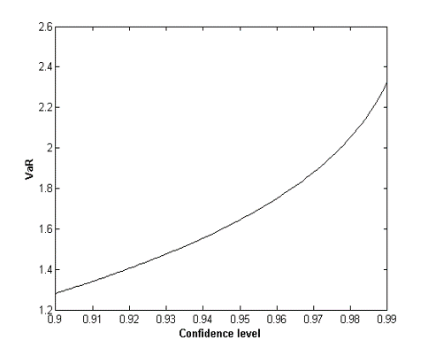
VaR rises with confidence level (cl) at an increasing rate

VaR Parameters: The Holding Period (hp)

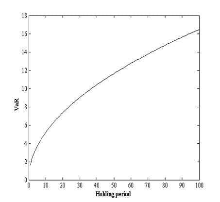
If mean is zero, VaR rises with square root of holding period
'Square root rule': $\small VaR(T\text{ days})=VaR(1\text{ day})\times\sqrt{T}$
- Daily innovations must be i.i.d. standard normal (why?)
Empirical plausibility of SRR very doubtful (why?)

VaR Surface

VaR surface is much more revealing
A single VaR number is just a point on the surface – doesn’t tell much
With zero mean, get spike at high cl and high hp

Determine the Confidence Level

High cl if we want to use VaR to set capital requirements
- E.g., 99% under Basel
Lower if we want to use VaR
- to set position limits
- for reporting/disclosure
- for backtesting (we will discuss it later)

Determine the Holding Period

Depends on investment/reporting horizons
Daily common for cap market institutions
10 days (or 2 weeks) for banks under Basel
Can depend on liquidity of market – hp should be equal to liquidation period
Short hp makes it easier to justify assumption of unchanging portfolio
Short hp preferable for model validation/backtesting requirements
- Short hp means more data to use

Marginal, Incremental, and Component Measures

Suppose that the amount invested in i-th subportfolio is $x_i$ . The marginal value at risk for the i-th subportfolio is the sensitivity of VaR to the amount invested in the i-th subportfolio.
$\frac{\partial{VaR}}{\partial x_i}$
The incremental value at risk for the ith subportfolio is the incremental effect of the ith subportfolio on VaR. It is the difference between VaR with the subportfolio and VaR without the subportfolio.
The component value at risk for the ith subportfolio is
$C_i=\frac{\partial VaR}{\partial x_i}x_i\approxeq\frac{\Delta VaR}{\Delta x_i}x_i$

Euler's Theorem

Suppose that $V$ is a risk measure for a portfolio and $x_i$ is a measure of the size of the i-th subportfolio ( $1\leq i\leq M$ ). Assume that, when $x_i$ is changed to $\lambda x_i$ for all $x_i$ (so that the size of the portfolio is multiplied by $\lambda$ ), $V$ changes to $\lambda V$ .
Euler's theorem shows that it is then true that
$V=\sum_{i=1}^M\frac{\partial V}{\partial x_i}x_1$
- for VaR:
  $VaR=\sum_{i=1}^MC_i$
- for ES:
  $ES=\sum_{i=1}^M\frac{\partial ES}{\partial x_i}x_1$

Limitation of VaR

VaR estimates subject to error
VaR models subject to (considerable!) model risk
- Beder
VaR systems subject to implementation risk
- Marshal and Siegel
But these problems common to all risk measurement systems

VaR uninformative of tail losses

VaR tells us most we can lose at a certain probability, i.e., if tail event does not occur
VaR does not tell us anything about what might happen if tail event does occur
Trader can spike firm by selling out of the money options
- Usually makes a small profit, occasionally a very large loss
- If prob of loss low enough, such a position appears to have no risk, but can be very dangerous
Two positions with equal VaRs not necessarily equally risky, because tail events might be very different
Solution to use more VaR information – estimate VaR at higher cl

VaR creates perverse incentives

VaR-based decision calculus can be misleading, because it ignores low-prob, high-impact events
- Events with probs less than VaR tail prob ignored
Additional problems if VaR is used in a decentralized system
VaR-constrained traders/managers have incentives to 'game' the VaR constraint
- Sell out of the money options, etc.

VaR can discourage diversification

VaR of diversified portfolio can be larger than VaR of undiversified one
Example
- 100 possible states, 100 assets, each making a profit in 99 (different) states, and a high loss in one
- Diversified portfolio is certain to experience a high loss
- Undiversified portfolio is not
- Hence, VaR of diversified portfolio higher than VaR of undiversified one

VaR not subadditive

A risk measure $\rho(\cdot)$ is subadditive if risk of sum is not greater than sum of risks
$\rho(A+B)\leq\rho(A)+\rho(B)$
Aggregating individual risks does not increase overall risk
Important because: Adding risks together gives conservative (over-) estimate of portfolio risk – want bias to be conservative
If risks not subadditive and VaR used to measure risk
- Firms tempted to break themselves up to release capital
- Traders on organized exchanges tempted to break up accounts
- In both cases, problem of residual risk exposure
Subadditivity is highly desirable
But VaR is only subadditive if risks are normal or elliptical
VaR not subadditive for arbitrary distributions

Example: Suppose each of two independent projects has a probability of 0.02 of a loss of $10 million and a probability of 0.98 of a loss of $1 million during a one-year period. The one-year, 97.5% VaR for each project is $1 million. When the projects are put in the same portfolio, there is a 0.02 × 0.02 = 0.0004 probability of a loss of $20 million, a 2 × 0.02 × 0.98 = 0.0392 probability of a loss of $11 million, and a 0.98 × 0.98 = 0.9604 probability of a loss of $2 million. The one-year 97.5% VaR for the portfolio is $11 million. The total of the VaRs of the projects considered separately is $2 million. The VaR of the portfolio is therefore greater than the sum of the VaRs of the projects by $9 million. This violates the subadditivity condition.

Example: A bank has two $10 million one-year loans. The probabilities of default are as indicated in the following table.

Outcome Probability

Neither loan defaults 97.50%

Loan 1 defaults; Loan 2 does not default 1.25%

Loan 2 defaults; Loan 1 does not default 1.25%

Both loans default 0.00%

If a default occurs, all losses between 0% and 100% of the principal are equally likely. If the loan does not default, a profit of $0.2 million is made.

Consider first Loan 1. This has a 1.25% chance of defaulting. When a default occurs the loss experienced is evenly distributed between zero and $10 million. This means that there is a 1.25% chance that a loss greater than zero will be incurred; there is a 0.625% chance that a loss greater than $5 million is incurred; there is no chance of a loss greater than $10 million. The loss level that has a probability of 1% of being exceeded is $2 million. (Conditional on a loss being made, there is an 80% or 0.8 chance that the loss will be greater than $2 million. Because the probability of a loss is 1.25% or 0.0125, the unconditional probability of a loss greater than $2 million is 0.8 × 0.0125 = 0.01 or 1%.) The one-year 99% VaR is therefore $2 million. The same applies to Loan 2.

Consider next a portfolio of the two loans. There is a 2.5% probability that a default will occur. As before, the loss experienced on a defaulting loan is evenly distributed between zero and $10 million. The VaR in this case turns out to be $5.8 million. This is because there is a 2.5% (0.025) chance of one of the loans defaulting and conditional on this event is a 40% (0.4) chance that the loss on the loan that defaults is greater than $6 million. The unconditional probability of a loss from a default being greater than $6 million is therefore 0.4 × 0.025 = 0.01 or 1%. In the event that one loan defaults, a profit of $0.2 million is made on the other loan, showing that the one-year 99% VaR is $5.8 million.

The total VaR of the loans considered separately is 2 + 2 = $4 million. The total VaR after they have been combined in the portfolio is $1.8 million greater at $5.8 million. This shows that the subadditivity condition is violated. (This is in spite of the fact that there are clearly very attractive diversification benefits from combining the loans into a single portfolio-particularly because they cannot default together.)

Outcome	Probability
Neither loan defaults	97.50%
Loan 1 defaults; Loan 2 does not default	1.25%
Loan 2 defaults; Loan 1 does not default	1.25%
Both loans default	0.00%

Coherent Measure of Risk

Coherent Risk Measures

Let $X_1$ and $X_2$ be future values of two risky positions. A coherent measure of risk should satisfy the following axioms
- Monotonicity: if $X_1\leq X_2$ , $\rho(X_1)\leq\rho(X_2)$
- Translation invariance: $\rho(X+k)=\rho(X)-k$
- Homogeneity: $\rho(bX)=b\rho(X)$
- Subadditivity: $\rho(X_1+X_2)\leq\rho(X_1)+\rho(X_2)$
Homogeneity and Monotonicity imply convexity, which is important
Translation invariance means that adding a sure amount to our end-period portfolio will reduce loss by amount added

Implications of coherence

Any coherent risk measure is the maximum loss on a set of generalized scenarios
- GS is set of loss values and associated probs
Maximum loss from a subset of scenarios is coherent
Outcomes of stress tests are coherent
- Coherence theory provides a theoretical justification for stress testing!
Coherence risk measures can be mapped to user’s risk preferences
Each coherent measure has a weighting function $\phi(\cdot)$ that weights loss values
$\phi(\cdot)$ can be linked to utility function (risk preferences)
Can choose a coherent measure to suit risk preferences

Alternative Measures of Risk: CVaR

The Conditional VaR (CVaR) is the expected loss, given a loss exceeding VaR
$CVaR=E[X|X<VaR_c(X)]=\frac{\int_{-\infty}^{VaR_c(X)}x\color{red}{f(x)}dx}{\color{red}{\int_{-\infty}^{VaR_c(X)}f(x)dx}}$
it is also called expected shortfall, tailed conditioal expectation, conditional loss, or expected tail loss
VaR tells us the most we can lose if a tail event does not occur, CVaR tells us the amount we expect to lose if a tail event does occur
CVaR is coherent

CVaR is better than VaR

Tell us what to expect in bad states
- VaR tells us nothing
CVaR-based decision rule valid under more general conditions than a VaR-based one
- CVaR rule valid under second-order stochastic dominance
- VaR rule valid under first-order stochastic dominance
- FOSD more stringent than SOSD
CVaR coherent, and therefore always subadditive
CVaR does not discourage risk diversification, VaR sometimes does
CVaR-based risk surface always convex
- Convexity ensures that portfolio optimization has a unique well-behaved optimum
- Convexity also enables problems to be solved easily using linear programming methods

Alternative Measures of Risk: Worst-case scenario analysis

This is the outcome of a worst-case scenario analysis (Boudoukh et al)
Can consider as high percentile of distribution of losses exceeding VaR
- Whereas CVaR is expected value of this distribution
WCSA is also coherent, produces risk measures bigger than CVaR

Alternative Measures of Risk: SPAN

Standard-Portfolio Analysis Risk (SPAN, CME)
Considers 14 scenarios (moderate/large changes in vol, changes in price) + 2 extreme scenarios
Positions revalued under each scenario, and the risk measure is the maximum loss under the first 14 scenarios plus 35% of the loss under the two extreme scenarios
SPAN risk measure can be interpreted as maximum of expected loss under each of 16 probability measures, and is therefore coherent

Alternative Measures of Risk: Other Methods

The Semistandard Deviation
$SG_L(X)=\sqrt{\frac{1}{N_L}\sum_{i=1}^N(x_i^-)^2}$
The Drawdown
$DD(X)=\frac{x^{\max}-x_t}{x^{\max}}$
Try to verify wether the following popular risk measures are coherent measures of risk or not
- Standard deviation
- VaR
- CVaR
- WCSA
- SPAN

Stress-Testing

What are stress tests?

STs are procedures that gauge vulnerability to 'what if' events
- Used for a long time, especially to gauge institutions IR exposure
Early stress tests 'back of envelope' exercises
Major improvements in recent years, helped by developments in computer power
Modern ST much more sophisticated than predecessors

Modern stress testing

ST received a major boost after 1998
Realisation that it would have helped firms to protect themselves better in '98 crisis'
ST very good for quantifying possible losses in non-normal situations
- Breakdowns in normal correlation relationships
- Sudden decreases in market liquidity
- Handling concentration risks
- Handling macroeconomic risks
STs versus probabilistic aprpoaches
- STs are a natural complement to probabilistic approaches
- VaR and CVaR good on prob side, but poor on 'what if'
- STs poor on prob side, but good on 'what if'
- STs not designed to answer prob questions

Categories of STs

Different types of event (normal, extreme, etc.)
Different types of risk (market, credit, etc.) and risk factors (equity risks, yield curve, etc.)
Different country/region factors
Different methodologies (scenario analysis, factor push, etc.)
Different assumptions (relating to yields, stock markets, etc.)
Different books (trading, banking)
Differences in level of test (firmwide, business unit, etc.)
Different instruments (equities, futures, options, etc.)
Differences in complexity of portfolio

Main types of stress test

Scenario ('what if') analysis
- Analyse impact of specific scenario on our financial position
Mechanical stress tests
- Evaluate a number of math/stat defined scenarios (e.g., defined in terms of movements in underlying risk factors)
- Work through these in a mechanical way

Uses of stress tests

Can provide good risk information
- Good for communicating risk information
- Results from STs readily understandable
- But must avoid swamping recipients with too much data
Can guide decision making
- Allocation of capital, setting of limits, etc.
ST can help firms to design systems to deal with bad events
- Can check on modelling assumptions, contingency planning, etc.

Benefits of stress testing

Good for showing hidden vulnerability
Can improve on VaR type information in various ways
- Since stress events unlikely, VaR systems unlikely to reveal much about them
- Short VaR holding period will often be too short to reveal full impact of stress event
- Stress tests better at handling non-linearities that arise in stress situations
- Stress test can take account of unusual features in a stress scenario
Can more easily identify a firm’s breaking point
- Identify lethal conjunctions of events, etc.
Can give a clearer view about dangerous scenarios
- This helps in deciding they might be handled
Stress tests particularly good for identifying and handling liquidity exposures
- Loss of liquidity a key feature of crises
Stress tests also very good for handling large market moves
- Market crashes, etc
Stress tests good for handling possible changes in market volatility
- Help identify possible risks in overall risk exposure, gains/losses on derivatives positions, etc
Stress tests for good for handling exposure to correlation changes
- These very significant in major crises
Stress tests good for highlighting hidden weaknesses in risk management system
- Identify hidden 'hot spots' in portfolio

Difficulties with STs

Much less straightforward than it looks
Based on large numbers of decisions about
- choice of scenarios and risk factors
- how risk factors should be combined
- Ranges of values to be considered
- Choice of time horizon, etc.
ST results completely dependent on chosen scenarios and how they are modelled
- When portfolios are complex, can be very difficult even to identify the risk factors to look at
Difficulty of working through scenarios in a consistent way
- Need to follow through scenarios, and consequences can be very complex and can easily become unmanageable
- Need to take account of interrelationships in a reasonable way
  - Need to account for correlations
- Need to take account of zero arbitrage relationships
  - Eliminate 'impossible' events?

ST & Prob Analysis

Interpretation of ST results
- STs do not address prob issues as such
- Hence, always an issue of how to interpret results
- This implies some informal notion of likelihood
  - If prob is negligible, result of ST might have little bearing
  - If prob is significant, result might be importan
Integrating ST and prob analysis
- Can integrate ST and prob analysis using Berkowitz’s coherent framework
  - Do prob analysis – VaRs at different cls
  - Do ST analysis
  - Assign probs to ST scenarios
  - Integrate these outcomes into prob analysis
- This approach is judgemental, but does give an integrated analysis of both probs and STs

Choosing scenarios

moving key variables one at a time
using historical scenarios
creating prospective scenarios
reverse stress tests

Stylised Scenarios

Simulated movement in major IRs, stock prices, etc.
- Can be expressed in absolute changes or multiple-of-std changes
Long been used in ALM analysis
Problem is to keep scenarios down in number, without missing plausible important ones

Actual Historical Scenarios

Based on actual historical events
Advantages
- They have plausibility because they have occurred
- Readily understood
Can choose scenarios from a catalogue, which might include
- Moderate market changes
- More extreme events such as reruns of major crashes
  - A good guide is to choose scenarios that are of same order of magnitude as worst-case events in our data sets

Hypothetical One-Off Events

These might be natural, political, legal, major defaults, counterparty defaults, economic crises, etc.
Can obtain them by alternate history exercises
- Rerun historical scenarios and ask what might have been
Can also look to historical record to guide us in working out what such scenarios might look like

Evaluating scenarios

Having specified our set of scenarios, we then need to evaluate their effects
Key is to get an understanding of the sensitivities of our positions to changes in the risk factors being changed
Easy for some positions
- E.g., linear FX, stock, futures positions
Harder for options
- Must account for (changing) sensitivities to underlying
- Might need approximations, e.g., delta-gamma
Must pay particular attention to impact of stylised events on markets
Very unwise to assume that liquidity will remain strong in a crisis
If futures contracts are used hedges, must also take account of funding implications
Otherwise well-hedged positions can unravel because of interim funding

Mechanical ST

These approaches try to reduce subjectivity of SA and put ST on firmer foundation
- Instead of using subjective scenarios, we use math/stat generated scenarios
- Work through these in a systematic way
- Work out most damaging conjunctions of events
Mechanical ST more systematic and thorough than SA, but also more intensive

Factor Push Analysis

Push each price or factor by a certain amount
- Better to push factors than prices, due to varying sensitivities of prices to factors
Specify confidence level $\alpha$
Push factors up/down by $\alpha$
Revalue positions each time,
Work out most disadvantageous combination
This gives us worst-case maximum loss (ML)
FP is easy to program, at least for simple positions
Does not require very restrictive assumptions
Can be modified for correlations,
Results of FP are coherent
If we are prepared to make further assumptions, FP can also give us an indication of likelihoods
- ML estimates tend to be conservative estimates of VaR
- Can adjust the $\alpha$ to obtain probs and VaRs
But FP rests on assumption that highest losses occur when factors move most, and this is not true for some positions

Maximum Loss Optimisation

Solution to this problem is to search over interim values of factor ranges
This is MLO
MLO is more intensive, but will pick up high losses that occur within factor ranges
- E.g., as with losses on straddles
MLO is better for more complex positions, where it will uncover losses that FP might miss

Backtesting（回顾测试）

Backtesting

Backtesting is the process to compare systematically the VaR forecasts with actual returns.
- It should detect weaknesses in the models and point to areas for improvement
- It is one of the reasons that bank regulators allow banks to use their own risk measures to determine the amount of regulatory capital
Backtesting compares the daily VaR forecast with the realized profit and loss (P&L) the next day.
- It is recorded as an exception（例外） if the actual loss is worse than the VaR
- The risk manager counts the number if exceptions $x$ over a window with $T$ observations.
Trading outcome
- Actual portfolio
- Hypothetical portfolio (no intraday trading, no fee income)
- The Basel framework recommends using both hypothestical and actual trading outcomes in backtests

Preparing Data: Obtaining Data

Need to obtain suitable P/L data
Accounting (e.g., GAAP) data often inappropriate because of smoothing, prudence etc
Want P/L data that reflect market risks taken
- Need to eliminate fee income, bid-ask profits, P/L from other risks taken (e.g., credit risks), unrealised P/L, provisions against future losses
Need to clean data or use hypothetical P/L data (obtained by revaluing periods from day to day)

Preparing Data: Draw up backtest chart

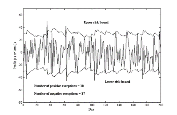
Good to plot P/L data against risk bounds over time
Chart good indicator of possible problems
- over-estimation of risks
- under-estimation of risks
- bias
- excessive smoothness in risk bounds, etc.

Preparing Data: Get to know data

Draw up summary statistics
- Mean, std, skewness, kutosis, min, max, etc.
Draw up QQ charts
- Plots of predicted vs. empirical quantiles
Draw up charts of predicted vs. empirical probs
Shape of these curves indicates whether supposed pdf fits the data – very useful diagnostic

Preparing Data: Standardise Data

P/L data typically random
Porfolios and dfs often change from day to day
How to compare P/L data if underlying pdfs change?
Good practice to map P/L data to predicted percentile
- If observation falls 90% percentile of predicted P/L distribution, then mapped value is 0.90
This standardizes data to make observations comparable given changes in pdf or porfolio

Measuring Exceptions

Binomial Distribution
- Probability mass function
  $f(x)=\binom{T}{x}p^x(1-p)^{T-x},\ x=0,1,2,\dots,T$
- Mean: $pT$ , Variance: $p(1-p)T$
Example: For instance, we want to know what is the probability of observing $x=0$ exceptions out of a sample of $T=250$ observations when the true probability is 1%. We should expect to observe $p\times T=2.5$ exceptions on average across many such samples. There will be, however, some samples with no exceptions at all simply due to luck. This probability is
$f(X=0)=\frac{T!}{x!(T-x)!}p^x(1-p)^{T-x}=\frac{250!}{1\times250!}0.01^00.99^{250}=0.081$
So, we would expect to observe 8.1% of samples with zero exceptions under the null hypothesis. We can repeat this calculation with different values for $x$ . For example, the probability of observing eight exceptions is $f (X =8) = {250 \choose 8}0.01^8(0.99)^{242}=0.02\%$ . Because this probability is so low, this outcome should raise questions as to whether the true probability is 1%.
Normal Approximation
$z=\frac{x-pT}{\sqrt{p(1-p)T}}\sim N(0,1)$
Decision Rule for Backtests
- Type 1 errors: kill the good guy
- Type 2 errors: miss the bad guy
- Power of a test is one minus the type 2 error rate
- Most statistical tests fix the type 1 error rate, say at 5%, and structure the test so as to minimize the type 2 error rate, or maximize the test's power

Example

Consider a VaR measure over a daily horizon defined at the 99% level of confidence $c$ . The window for backtesting is $T=250$ days.

A higher cutoff point would lower the type 1 error rate
It is more likely to miss VaR models that are misspecified with higher cutoff points

Basel Rule for Backtests

The normal multiplier $k$ for capital charge is 3
After an incursion into the yellow zone $k$ is increased to $4$ according to the table
An incursion into the red zone generates an automatic, non-discretionary penalty

Evaluation of Backtesting

Exception tests focus only on the frequency of occurrences
It ignores the time pattern of losses

Advanced Risk Models: Multivariate

The Big Idea

Components of a Multivariate Risk Modeling Systems

Risk system
- portofolio position system
- risk factor modeling system
- aggregation system
Describe joint movements in the risk factors
- specify an analytical distribution
- take the joint distribution from empirical observations
Aggregation: VaR methods
- delta-normal method
- historical simulation method
- Monte Carlo simulation method

Risk Mapping

Introduction

Have assumed so far that each position has its own risk factor, which we model directly
- Distinguish between positions and risk factors
However, it is not always possible or desirable to model each position as having its own risk factor
Might wish to map our positions onto some smaller set of risk factors
- Might wish to map $n$ positions to $m$ ( $<n$ ) risk factors

Reasons for mapping

Might not have enough data on our positions
- E.g., might have small runs of Emerging Market data
- Map to risk factors for which we do have data
Might wish to cut down on the dimensionality of our covariance matrices
- This is important!
- With $n$ positions, covariance matrix has $n(n+1)/2$ terms
- As $n$ rises, covariance matrix becomes more unwieldy
Need to keep dimensionality down to avoid computational problems too – rank problems, etc.

Stages of mapping

Construct a set of benchmark instruments or factors
- Might include key bonds, equities, etc.
Collect data on their volatilities and correlations
Derive synthetic substitutes for our positions, in terms of these benchmarks
- This substitution is the actual mapping
Construct VaR/CVaR of mapped porfolio
Take this as a measure of the VaR/CVaR of actual portfolio

Selecting Core Instruments

Usual approach to select key core instruments
- Key equity indices, key zero bonds, key currencies, etc.
Want to have a rich enough set of these proxies, but don’t want so many that we run into covariance matrix problems
RiskMetrics core instruments
- Equity positions represented by equivalent amounts in key equity indices
- Fixed income positions by represented by combinations of cashflows of a limited number of maturities
- FX positions represented by relevant amounts in `core' currenicies
- Commodity positions represented by amounts of selected standardised futures positions

Mapping with Principal Components

Can use PCA to identify key factors
Small number of PCs will explain most movement in our data set
PCA can cut down dramatically on dimensionality of our problem, and cut down on number of covariance terms
- E.g., with 50 original variables, have $50(51)/2=1275$ separate covariance terms
- With 3 PCs, have only 3 separate covariance terms

Mapping Positions to Risk Factors

Most positions can be decomposed into primitive building blocks
Instead of trying to map each type of position, we can map in terms of portfolios of building blocks
Building blocks are
- Basic FX
- Basic equity
- Basic fixed-income
- Basic commodity

A General Example of Risk Mapping

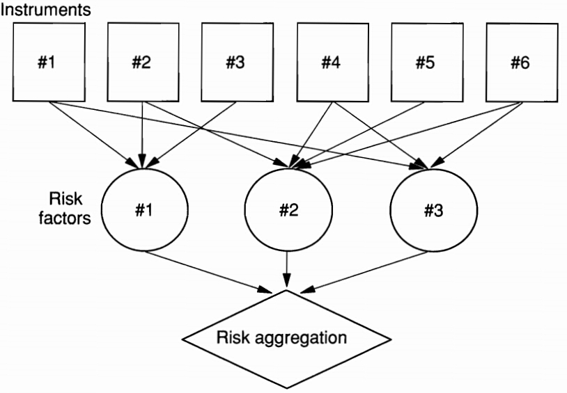
Replace each if the $N$ positions with a $K$ exposure on the risk factors. Define $x_{i,k}$ as the exposure of instruments $i$ to risk factor $k$
Aggregate the $K$ exposures across the positions in the portfolio, $x_k=\sum_{i=1}^Nx_{i,k}$
Derive the distribution of the portfolio return $R_{p,t+1}$ from the exposures and movements in risk factors, $\Delta f$ , using one of the three VaR methods

Example: Mapping with Factor Models

Decompose stock return $R_i=\alpha_i+\beta_i\times R_M+\epsilon_i$
- a constant term (not important fot risk management purpose)
- a component due to the market $R_M$
- a residual term
The portfolio return
- Mean: $R_p=\sum_{i=1}^Nw_iR_i=\beta_pR_M+\sum_{i=1}^Nw_i\epsilon_i$
- Variance: $V[R_p]=\beta^2_pV[R_M]+\sum_{i=1}^Nw_i^2V[\epsilon_i]$
- For equally weighted portfolio: $\sum_{i=1}^Nw_i^2V[\epsilon_i]\rightarrow N\times\frac{V}{N^2}=\frac{V}{N}$
- The mapping: $x_i$ on stock $i\rightarrow(x_i\beta_i)$ on index
This approach is useful especially when there is no return history

Example: Mapping with Fixed-Income Portfolios

Risk-free bond portfolio
- maturity mapping: replace the current value of each bond by a position on a risk factor with the same maturity
- duration mapping: maps the bond on a zero-coupon risk factor with a maturity equal to the duration of the bond
- cash flow mapping: maps the current value of each bond payment on a zero-coupon risk factor with maturity equal to the time to wait for each cash flow
Corporate bond portfolio
- Decomposition: $y_i=z_j+s_k+\epsilon_i$
- the movement in the value of bond price $i$ :
  $\Delta P_i=-DVBP_i\Delta y_i=-DVBP_i\Delta z_j-DVBP_i\Delta s_k-DVBP_i\Delta\epsilon_i$
the portfolio: $P=\sum_{i=1}^Nn_iP_i$
aggregation:
$\begin{array}{lll} \Delta P&=&\sum_{i=1}^Nn_i\Delta P_i=-\sum_{i=1}^Nn_iDVBP_i\Delta y_i &=&-\sum_{j=1}^JDVBP_j^z\Delta z_j-\sum_{j=k}^KDVBP_k^s\Delta s_k-\sum_{i=1}^Nn_iDVBP_i\Delta \epsilon_i \end{array}$
Variance: $V[\Delta P]=\text{General Risk}+\sum_{i=1}^Nn^2_iDVBP_i^2V[\Delta\epsilon_i]$
$x_i$ on bond $i\rightarrow(n_iDVBP_i)$ on $yield_j +(n_iDVBP_i)$ on $spread_k$

Choice of Risk Factors

It should be driven by the nature of the portfolio:

portfolio of stocks that have many small positions well dispersed across sectors
portfolios with a small number of stocks concentrated in one sector
an equity market-neutral portfolio
$\dots$

Mapping Complex Positions

Complex positions are handled by apply financial engineering theory
Reverse-engineer complex positions into portfolios of simple positions
Map complex positions in terms of collections of synthetic simple positions
Some examples, using FE/FI theory:
- Coupon-paying bonds: can regard as portfolios of zeros
- FRAs: equivalent to spreads in zeros of different maturities
- FRNs: equivalent to a zero with maturity equal to period to next coupon payment (because it reprices at par)
- Vanilla IR swaps: equivalent to portfolio long a fixed-coupon bond and short a FRN
- Structured notes: equivalent to combinations of IR swaps and conventional FRNs
- FX forwards: equivalent to spread between foreign currency bond and domestic currency bond
- Commodity, equity and FX swaps: combinations of spread between forward/futures and bond position

Dealing with Optionality

All these positions can be mapped with linear based mapping systems because of their being (close to) linear
These approaches not so good with optionality
- Non-linearity of options positions can lead to major errors in mapping
With non-linearity, need to resort to more sophisticated methods, e.g., delta-gamma and duration-convexity

Joint Distribution of Risk Factors

Copula

Copula is a function of the values of the marginal distributions $F(x)$ plus some parameters, $\theta$ , that are specific to this function. For example, $c_{12}[F_1(x_1),F_2(x_2);\theta]$
Sklar's theorem: For any joint density there exists a copula that links the marginal densities:
$f_{12}(x_1,x_2)=f_{1}(x_1)\times f_{2}(x_2)\times c_{12}[F_1(x_1),F_2(x_2);\theta]$
This result enables us to construct joint density functions from the marginal density functions and the copula function
Takes account of dependence structure
To model joint density function, specify marginals, choose copula, and then apply copula function

Common Copulas

Independence (product) copula $= uv$
- Good for independent random variables
Minimum copula $= \min(u,v)$
- Good for comonotonic variables
Maximum copula $= \max(u+v-1,0)$
- Good for countermonotonic variables
Gaussian copulas
- For multi-variable normality, does not have closed form copula functions
t-copulas
- For multi-variable $t$
Gumbel copulas, Archimedean copulas
Extreme value copulas
- Arising from EVT

Tail Dependence

Tail dependence
- Upper & lower conditional probabilities
  $\begin{array}{lll} P_U(c)&=&P[X_2>F_{X_2}^{-1}(c)|X_1>F_{X_1}^{-1}(c)] P_L(c)&=&P[X_2\leq F_{X_2}^{-1}(c)|X_1\leq F_{X_1}^{-1}(c)] \end{array}$
- When $P_U(c)$ and $P_L(c)$ approaches zero as $c\rightarrow0$ , a copula is said to exhibit tail independence
Gives an idea of how one variable behaves in limit, given high value of another

Extreme Value Theory

Peaks Over Threshold Approach & the GP Distribution

The limit distribution for values $x$ beyond a cutoff point $u$ ( $y=\frac{x-u}{\beta}$ ) belongs to the following family

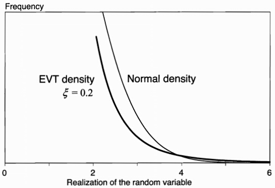
$\begin{array}{lll} f(y)=\left\{\begin{array}{ll} 1-(1+\xi y)^{1/\xi}, & \xi\neq0\\ 1-\exp(-y), & \xi=0 \end{array}\right. \end{array}$

It is called the generalized Pareto (GP) distribution
- $\beta>0$ is the scale parameter
- $\xi$ is the shape parameter that determines the speed at which the tail disappears
- EVT distribution is only asymptotically valid (i.e., as $u$ grows large)
It subsumes other distributions as special cases
- $\xi=0$ : normal distribution
- $\xi\rightarrow0$ : Gumbel
- $\xi>0$ : Fr'{e}chet (fat tails)
- $\xi<0$ : Weibull

Block Maxima vs. Peaks over Threshold

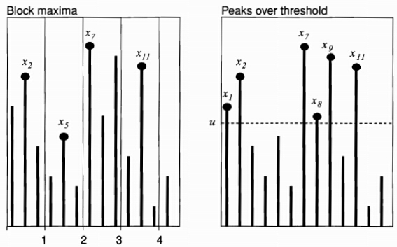
Block maxima approach: group the sample into successive blocks, from which each maximum is identified.
Generalized extreme value (GEV) distribution

EVT vs. Normal Densities

VaR and EVT

Close-form solutions for VaR and CVaR rely heavily on the estimation of $\xi$ and $\beta$ .

Maximum likelihood
- define a cutoff point $u$ (include 5% of the data in the tail)
- only consider losses beyond $u$ and maximize the likelihood of the observations over the two parameters $\xi$ and $\beta$
Method of moments
- fitting the parameters so that the GP moments equal the observed moments
Hill's estimator
- sort all observations from highest to lowest
- tail index is estimated from $\hat{\xi}=\frac{1}{k}\sum_{i=1}^k\ln X_i-\ln X_{k+1}$
- no theory tells how to choose $k$
- we may plot $\xi$ against $k$ and choose the value in a flat area

Problems with EVT

Estimates are sensitive to changes in the sample
Results depend on assumptions and estimation method
It relies on historical data

VaR Methods

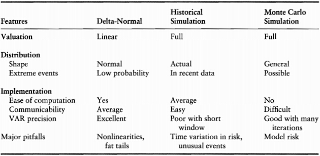
Delta-Normal

Assumption
- portfolio exposures are linear
- risk factors are jointly normally distributed
The VaR
- portfolio return is normally distributed
- the portfolio variance: $\sigma^2(R_{p,t+1})=x_t'\Sigma_{t+1}x_t$
- VaR is directly obtained from the standard normal deviate $\alpha$ that corresponds to the confidence level $c$ :
  $VaR=\alpha(c)\sigma(R_{p,t+1})$
- diversified VaR vs. undiversified VaR
Advantages & Drawbacks
- advantages: simple, closed-form, more precise, less sampling variability
- drawbacks: can not account for nonlinear effects (option), underestimate the occurrence of large observations (normal assumption)

Historical Simulation

The Idea: replays a ''tape'' of history to current positions
- go back in time (e.g. over the past 250 days)
- project hypothetical factor values using the factor movements
- derive the portfolio values
The VaR
- current portfolio value as function of current risk factors: $P_t=P(f_{1,t},f_{2,t},\dots,f_{N,t})$
- sampling factor movements from the historical distribution: $\Delta f_i^k=\{\Delta f_{i,1},\Delta f_{i,2},\dots,\Delta f_{i,t}\}$
- construct hypothetical factor values: $f_i^k=f_{i,t}+\Delta f_i^k$
- current portfolio value: $P^k=P(f_1^k,f_2^k,\dots,f_N^K)$
- portfolio return: $R^k=\frac{P^k-P_t}{P_t}$
- VaR is obtained from the difference between the average and the \textit{c}th quantile: $VaR=Ave(R_p)-R_p(c)$
Advantages & Drawbacks
- advantages: no specific distributional assumption, intuitive
- drawbacks: its reliance on a short historical moving window to infer movements in market prices

Monte Carlo Simulation

The Idea
- is similar to the historical simulation method
- the movements in risk factors are generated from a prespecified distribution: $\Delta f^k\sim g(\theta),\ k=1,\dots,K$
- the risk manager needs to specify the marginal distribution of risk factors as well as their copula
Advantages & Drawbacks
- advantages: most flexible
- drawbacks: computational burden, subject to model risk, sampling variability
It should converge to the delta-normal VaR if all risk factors are normal and exposures are linear

Comparison of Methods

Limitations of Risk Systems

Illiquid Assets
Losses Beyond VaR
Issues with Mapping
Reliance on Recent Historical Data
Procyclicality
Crowded Trades

课堂练习

A、B两只股票最近30周的周回报率如下所示（单位：1%）：

A: -3，2，4，5，0，1，17，-13，18，5，10，-9，-2，1，5，-9，6，-6，3，7，5，10，10，-2，4，-4，-7，9，3，2；

B: 4，3，3，5，4，2，-1，0，5，-3，1，-4，5，4，2，1，-6，3，-5，-5，2，-1，3，4，4，-1，3，2，4，3。

某金融机构用A、B按1：1比例构造投资组合。

(a) 请分别计算组合在90%置信水平下的VaR和CVaR。
(b) 通过计算验证VaR和CVaR是否为相容风险度量(coherent measure of risk)。

课堂练习

某交易组合是由价值300,000美元的黄金投资和价值500,000美元的白银投资构成，假定以上两资产的日波动率分别为1.8%和1.2%，并且两资产回报的相关系数为0.6，请问：（ $\Phi(1.96)=0.975$ ）

(a) 交易组合10天展望期的97.5%VaR为多少？
(b) 投资分散效应减少的VaR为多少？

课堂练习

假设我们采用100天的数据来对VaR进行回顾测试，VaR所采用的置信水平为99%，在100天的数据中我们观察到5次例外。如果我们因此而拒绝该VaR模型，犯第一类错误的概率为多少？