L01 Introduction & Preliminaries

• L01 Introduction & Preliminaries
  • Introduction to Financial Instruments
    • Interest Rate & Bond Fundamentals
      • Compound Interest
      • Zero Rates
      • Bond Pricing
      • Bound Yield
      • (Macaulay's) Duration
      • Modified Duration
      • Bond Portfolios
      • Convexity
    • Equities
      • Gordon Growth Model
      • Systematic Risk & Nonsystematic Risk
      • Measuring Systematic Risk: Beta
      • CAPM: The Security Market Line (SML)
      • Arbitrage Pricing Theory (APT)}
      • Understanding APT
      • Forwards and Futures
      • Pricing: No-arbitrage Argument}
      • Option
      • Payoff (Diagram)
      • Option Pricing: The Black-Scholes Formula
      • Understanding Black-Scholes
  • Introduction to Financial Risk Mamagement
    • Managing Linar Risk
      • Hedge}
      • Hedge Horizon and Contract Maturity
      • Basis Risk
      • Long Hedge
      • Short Hedge
      • Choice of Contract
      • Cross Hedging
      • Tailing the Hedge}
      • Example
      • Hedging Using Index Futures
      • Changing $\beta$
      • Example
    • Nonlinear (Option) Risk Models
      • Option Sensitivities

Introduction to Financial Instruments

Interest Rate & Bond Fundamentals

Compound Interest

• Elements of Compound Interest
  • frequency of compounding
  • the rate

$$A\left(1+\frac{R_m}{m}\right)^{mn}$$

• Continuous Compounding
  $$\lim_{m\rightarrow\infty}A\left(1+\frac{R}{m}\right)^{mn}=Ae^{Rn}$$

Zero Rates

• The $n$-year zero-coupond interest rate is the rate of interest earned on an investment that starts today and lasts for $n$ years. The investment provides payoff only at the end of year $n$.

  • e.g. a 5-year zero rate with continuous compounding quoted as 5% per annum

• It is also called $n$-year spot rate, $n$-year zero rate, and $n$-year zero.

• Most of the interest rate we observe directly in the market are not pure zero rate.

  • e.g. a 5-year government bond that provide 6% coupond

Bond Pricing

The idea: To calculate the cash price of a bond we discount each cash flow at the appropriate zero rate.

The Pricing Formula
$$B=\left\{\begin{array}{ll} \sum_{t=1}^{T}\frac{C_{t}}{\left(1+R_{t}\right)^{t}}+\frac{F}{\left(1+R_{T}\right)^{T}} & \text{(simple interest)}\\ \sum_{t=1}^{T}C_{t}e^{-R_tt}+Fe^{-R_TT} & \text{(continuously compounded)} \end{array}\right.$$
Example: A 2-year Treasure bond with a principal if $100 provides coupon at the rate of 6% per annum semiannually. The zero rates are quoted with continuous pompounding.

Maturity (years)	Zero rate (%)
0.5	5.0
1.0	5.8
1.5	6.4
2.0	6.8

$$3e^{-0.05\times0.5}+3e^{-0.058\times1.0}+3e^{-0.064\times1.5}+103e^{-0.068\times2.0}=98.39$$

Bound Yield

Bond yield is the single discount rate that, when applied to all cash flows, gives a bond price equal to its market price.
$$B=\sum_{t=1}^{T}C_{t}e^{-ty}+Fe^{-Ty}$$

Example: Suppose the market price of the bond is $98.39, please determine the yield to maturity.

$$3e^{-y\times0.5}+3e^{-y\times1.0}+3e^{-y\times1.5}+103e^{-y\times2.0}=98.39$$
Solving $y$, we have $y=6.76\%$.

(Macaulay's) Duration

• Duration is a measure of how long on average the holder of the bond has to wait before receiving cash payments.
• If the bond is priced as $B=\sum_{t=1}^Tc_te^{-yt}$ ($c_T$ is the sum of the last coupond and the face value), the duration is defined as
  $$D=\frac{\sum_{t=1}^Ttc_te^{-yt}}{B}=\sum_{i=1}^Tt\color{red}{\left[\frac{c_te^{-yt}}{B}\right]}$$
• Linear approximation: $\frac{\color{red}{\Delta B}}{B}\approx\frac{1}{B}\color{red}{\frac{dB}{dy}\Delta y}=-D\Delta y$
• Duration measures the sensitivity of bond price to the interest (discount) rate
• $DB$ is called the Dollar Duration, $DVBP=0.0001\times DB$ is the Dollar Value of a Basis Point

Modified Duration

Modified Duration is defined as $D^*=\frac{D}{1+y/m}$. It allows us to simplify $\Delta B$.

Generally, if $y$ is expressed with a compounding frequency of $m$ times per year, then

$$\Delta B=-\frac{BD\Delta y}{1+y/m}=-BD^*\Delta y$$

Bond Portfolios

• The duration for a bond portfolio is the weighted average duration of the bonds in the portfolio with weights proportional to prices
• The key duration relationship for a bond portfolio describes the effect of small parallel shifts in the yield curve
• What exposures remain if duration of a portfolio of assets equals the duration of a portfolio of liabilities?

Convexity

A measure of convexity is
$$C=\frac{1}{B}\frac{d^2B}{dy^2}=\frac{\sum_{i=1}^nc_it_i^2e^{-yt_i}}{B}$$

Approximate $\Delta B$ with the first two oder derivatives of the interest rate.
$$\frac{\Delta B}{B}=-D\Delta y+\frac{1}{2}C(\Delta y)^2$$
When used for bond portfolios it allows larger shifts in the yield curve to be considered, but the shifts still have to be parallel

Equities

Gordon Growth Model

• Assumptions

  • A firm pays out a dividend of $D$ over the next year
  • Dividends are expected to grow at the constant rate of $g$
  • Ignoring the final stock value
  • Discout rate $r>g$

• Model:
  $$P=\sum_{t=1}^{\infty}\frac{D(1+g)^{t-1}}{(1+r)^t}=\frac{D}{1+r}\sum_{t=0}^{\infty}\left(\frac{1+g}{1+r}\right)^t=\frac{D}{r-g}\nonumber$$

• In practice

  • Growth rate of dividends is uncertain
  • What is the required discount rate?
  • Some companies do not pay any divident

Systematic Risk & Nonsystematic Risk

• Systematic risk is risk that cannot be avoided and is inherent in the overall market.
  • It is also known as non-diversifiable or market risk
  • It is not diversifiable.
  • Examples of factors that constitute systematic risk include interest rates, inflation, economic cycles, political uncertainty, and widespread natural disasters.
• Nonsystematic risk is risk that is local or limited to a particular asset or industry
  that need not affect assets outside of that asset class.
  • It is also known as company-specific, industryspecific, diversifiable, or idiosyncratic risk.
  • It can be diversified.
  • Examples of nonsystematic risk could include the failure of a drug trial, major oil discoveries, or an airliner crash.
• How two manage these two classes of risks? (hedging / diversification)
• Pricing the risk (Systematic & Nonsystematic)

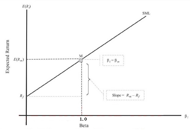
Measuring Systematic Risk: Beta

The Market Model: $R_i=\alpha_i+\beta_iR_m+e_i$. We have,
$$\begin{array}{lll} Cov(R_i,R_m)&=&Cov(\alpha_i+\beta_iR_m+e_i,R_m)\\ &=&Cov\left(R_f\left(1-\beta_i\right)+\beta_iR_m+e_i,R_m\right)\nonumber\\ &=&\beta_iCov(R_m,R_m)+\beta_iCov(e_i,R_m)\nonumber\\ &=&\beta_i\sigma_m^2 \end{array}$$
So, theoretically the beta can be calculated as below.
$$\beta_i=\frac{\sigma_{i,m}^2}{\sigma_m^2}=\frac{\sigma_i}{\sigma_m}\rho_{i,m}\nonumber$$

• Beta captures an asset's systematic risk, or the portion of an asset's risk that cannot be eliminated by diversification.
• What is the possible range of $\beta$?
• Try to calculate the beta for market portfolio & risk-free asset

CAPM: The Security Market Line (SML)

$$E[R_i]-R_f=\beta_i(E[R_m]-R_f)$$

Arbitrage Pricing Theory (APT)}

• CAPM is criticized because of the difficulties in selecting a proxy for the market portfolio as a benchmark

• An alternative pricing theory with fewer assumptions was developed: Arbitrage Pricing Theory (APT)

• Three Major Assumptions of Arbitrage Pricing Theory

  • Capital markets are perfectly competitive
  • Investors always prefer more wealth to less wealth with certainty
  • The stochastic process generating asset returns can be expressed as a linear function of a set of K factors or indexes

• APT does not assume

  • A market portfolio that contains all risky assets, and is mean-variance efficient
  • Normally distributed security returns
  • Quadratic utility function

• In application of the theory, the factors are not identified

• Similar to the CAPM, the unique effects are independent and will be diversified away in a large portfolio

• APT assumes that, in equilibrium, the return on a zero-investment, zero-systematic-risk portfolio is zero when the unique effects are diversified away

The expected return on any asset $i$ ($E[R_i]$) can be expressed as:
$$E[R_i]=\lambda_0+\lambda_1b_{i1}+\lambda_1b_{i2}+\dots++\lambda_1b_{ik}\text{ (APT)}$$

• $\lambda_0$: the expected return on an asset with zero systematic risk
• $\lambda_j$: the risk premium related to the jth common risk factor
• $b_{ij}$: the pricing relationship between the risk premium and the asset; that is; how responsive asset $i$ is to the $j$th common factor. (These are called factor betas or factor loadings.)

Understanding APT

• Arbitrage

  • No initial investment: $\sum_{i=1}^n\omega_i=0$ (in vector form $\omega'\vec{1}=0$)
  • Risk-free: $\sum_{i=1}^n\omega_i\beta_{ij}=0$ for $j=1,2,\dots,k$ (in vector form $\omega'\vec{\beta_j}=0$)
  • Positive profit: $\sum_{i=1}^n\omega_iE[r_i]>0$

• No-arbitrage: If $\text{(a)}+\text{(b)}\Longrightarrow\sum_{i=1}^n\omega_iE[r_i]=0$ (in vector form $\omega'E[\vec{r}]=0$), then
  $$E[r_i]=\lambda_0+\sum_{j=1}^k\lambda_j\beta_{i,j},\ \forall i=1,2,\dots,n$$

• A little math

  • Geometry: Normal and hyperplane
  • Riesz representation theorem

Forwards and Futures

• Forward Contract: A contract that obligates the holder to buy or sell an asset for a predetermined delivery price at a predetermined future time

  • Forward Price: The delivery price in a forward contract that causes the contract to be worth zero

• Futures Contract: A contract that obligates the holder to buy or sell an asset for a predetermined delivery price during a specified future time period. The contract is settled daily.

  • Futures Price: The delivery price currently applicable to a futures contract

• Forwards vs. Futures

FORWARDS	FUTURES
Private contracts between 2 parties	Traded on an exchange
Not standardized	Standardized contracts
Usually on specified delivery date	Range of delivery dates
Settled at end of contracts	Settled daily
Delivery or final cash settlement usually takes place	Contracts usually closed out prior to maturity
Some credit risk	Virtually no credit risk

Pricing: No-arbitrage Argument}

• The Big Idea: No arbitrage opportunity exists in an equilibium

• If a forward contract is underpriced, an investor can

  • Arbitrage by buying forward and selling spot
  • Her profit will be $S_0e^{rT}-F$

• If a forward contract is overpriced, an investor can

  • Arbitrage by buying spot and selling forward
  • Her profit will be $F-S_0e^{rT}$

• No (positive) profit is allowed, so we have
  $$\left\{\begin{array}{l} S_0e^{rT}-F\leq0\\ F-S_0e^{rT}\leq0 \end{array}\right.\Longrightarrow \color{red}{F=S_0e^{rT}}\nonumber$$

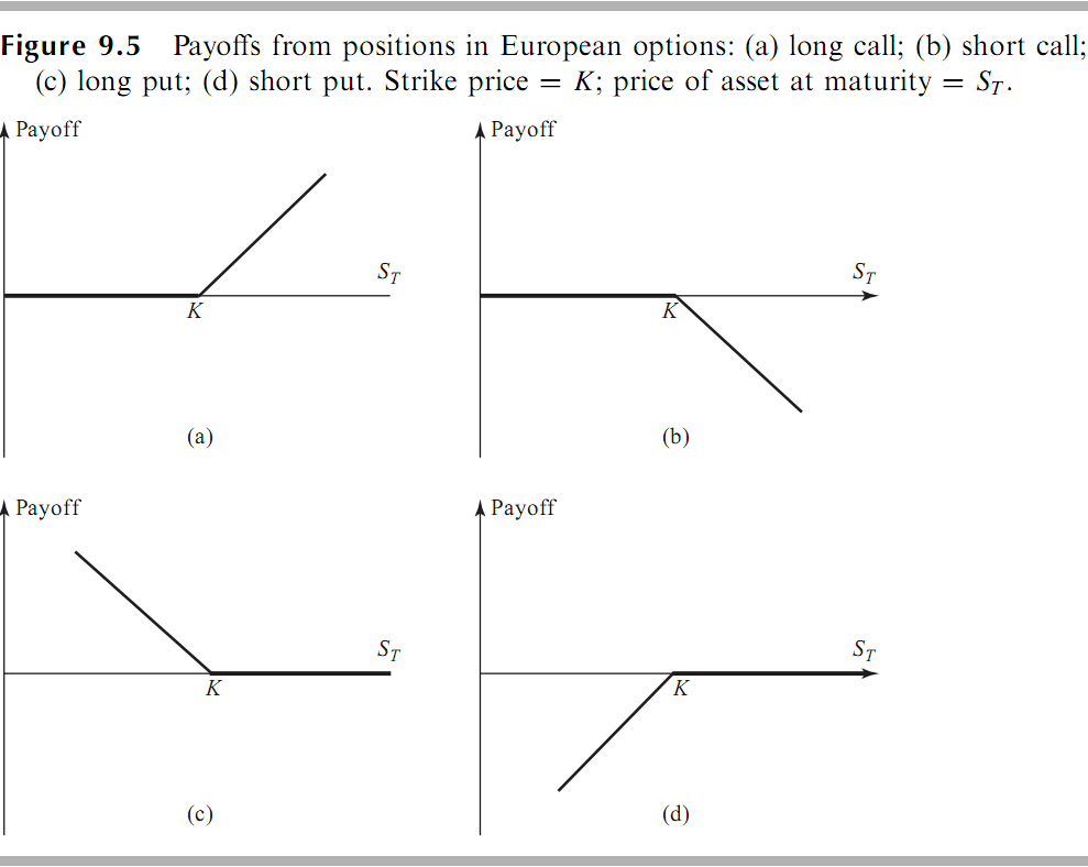
Option

An option is a contract which gives the buyer (the owner) the right, but not the obligation, to buy or sell an underlying asset or instrument at a specified strike price on or before a specified date.

• Underlying Assets: Stocks, Foreign Currency, Stock Indices, Futures

• Call vs. Put

  • A call option is an option to buy a certain asset by a certain date for a certain price, i.e. the strike price
  • A put option is an option to sell a certain asset by a certain date for a certain price, i.e. the strike price

• European vs. American

  • A European option can be exercised only at maturity
  • An American option can be exercised at any time during its life

• Excercise Price (Strike Price) & Expiration Date (Maturity Date)

• Options vs. Futures / Forwards

  • A futures/forward contract gives the holder the obligation to buy or sell at a certain price
  • An option gives the holder the right to buy or sell at a certain price

Payoff (Diagram)

	call	put
long	$\max(S_T-K,0)$	$\max(K-S_T,0)$
short	$-\max(S_T-K,0)$	$-\max(K-S_T,0)$

Option Pricing: The Black-Scholes Formula

• Geometric Brownian Motion
  $$\frac{dS}{S}=\mu dt+\sigma dZ$$
• The Black-Scholes-Merton Differential Equation is
  $$\frac{\partial f}{\partial t}+rS\frac{\partial f}{\partial S}+\frac{1}{2}S^2\frac{\partial^2 f}{\partial S^2}=rf$$
• Price of European call and put
  $$c=S_0N(d_1)-Ke^{-r\tau}N(d_2)$$
  $$p=Ke^{-r\tau}N(-d_2)-S_0N(d_1)$$
  where
  $$d_1=\frac{\ln(S_0/K)+(r+\sigma^2/2)\tau}{\sigma\sqrt{\tau}}$$
  $$d_2=\frac{\ln(S_0/K)+(r-\sigma^2/2)\tau}{\sigma\sqrt{\tau}}=d_1-\sigma\sqrt{\tau}$$

Understanding Black-Scholes

The formula
$$c=e^{-rT}N(d_2)\left(S_0e^{rT}N(d_1)/N(d_2)-K\right)$$
- $e^{-rT}$: Discount factor
- $N(d_2)$: Probability of exercise
- $e^{rT}N(d_1)/N(d_2)$: Expected percentage increase in stock price if option is exercised
- $K$: Strike price paid if option is exercised

Introduction to Financial Risk Mamagement

Managing Linar Risk

Hedge}

• Perfect hedging: the one that completely eliminates the risk

• A long futures hedge (involves a long position in future contract) is appropriate when you know you will purchase an asset in the future and want to lock in the price

• A short futures hedge (involves a short position in future contract) is appropriate when you know you will sell an asset in the future and want to lock in the price

Hedge Horizon and Contract Maturity

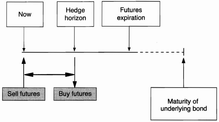
Basis Risk

• Problems give rise to what is termed basis risk

  • The asset whose price is to be hedged may not be exactly the same as the asset underlying the futures contract
  • The hedger may be uncertain as to the exact date when the asset will be bought or sold
  • The hedge may require the futures contract to be closed out before its delivery month

• Basis is the difference between the spot and futures price

• Basis risk arises because of the uncertainty about the basis when the hedge is closed out

Long Hedge

• We define
  $F_1$ : Initial Futures Price
  $F_2$ : Final Futures Price
  $S_2$ : Final Asset Price

• If you hedge the future purchase of an asset by entering into a long futures contract then
  $$\text{Cost of Asset}=S_2 - (F_2 - F_1) = F_1 + \text{Basis}$$

Short Hedge

• We define
  $F_1$ : Initial Futures Price
  $F_2$ : Final Futures Price
  $S_2$ : Final Asset Price

• If you hedge the future sale of an asset by entering into a short futures contract then
  $$\text{Price Realized}=S_2 + (F_1 - F_2) = F_1 + \text{Basis}$$

Choice of Contract

• Choose a delivery month that is as close as possible to, but later than, the end of the life of the hedge

• When there is no futures contract on the asset being hedged, choose the contract whose futures price is most highly correlated with the asset price. This is known as cross hedging.

Cross Hedging

• Cross hedging occurs when the two assets are different

• Hedge ratio is the size of position taken in futures contracts to the size of the exposure

• If we hedge the risk of one unit of the exposure with $h$ futures, the total change in the value of the portfolio is $\Delta V=\Delta S+h\Delta F$

• The total variance is $\sigma_{\Delta V}^2=\sigma_{\Delta S}^2+h^2\sigma_{\Delta F}^2+2h\sigma_{\Delta S}\sigma_{\Delta F}$

• Minimum variance hedge ratio
  $$h^*=-\rho\frac{\sigma_{\Delta S}}{\sigma_{\Delta F}}$$
  $\rho$ is the coefficient of correlation between $\Delta S$ and $\Delta F$.

Tailing the Hedge}

• Two way of determining the number of contracts to use for hedging are

  • Compare the exposure to be hedged with the value of the assets underlying one futures contract
    $$N^*=\frac{h^*Q_A}{Q_F}$$
  • Compare the exposure to be hedged with the value of one futures contract (=futures price time size of futures contract
    $$N^*=\frac{h^*V_A}{V_F}$$

• The second approach incorporates an adjustment for the daily settlement of futures

Example

An airline knows that it will need to purchase 10,000 metric tons of jet fuel in three months. It wants some protection against an upturn in prices using futures contracts.

The company can hedge using heating oil futures contracts traded on NYMEX. The notional for one contract is 42,000 gallons. As there is no futures contract on jet fuel, the risk manager wants to check if heating oil could provide an efficient hedge instead. The current price of jet fuel is $277/metric ton. The futures price of heating oil is $0.6903/gallon. The standard deviation of the rate of Change in jet fuel prices over three months is 21.17%, that of futures is 18.59%, and the correlation is 0.8243.

Compute:

1. The notional and standard deviation of the unhedged fuel cost in dollars

2. The optimal number of futures contract to buy/sell, rounded to the closest integer

Solution：

1. The position notional is $Q_S=\$2,770,000$. The standard deviation in dollars is
   $$\sigma(\Delta s/s)sQ=0.2117\times\$277\times10,000=\$586,409$$
   For reference, that of one futures contract is
   $$\sigma(\Delta f/f)fQ_f=0.1859\times\$0.6903\times42,000=\$5,389.72$$
   with a future notional of $Q_f=\$0.6903\times42,000=\$28,992.60$.

2. The cash position corresponds to a payment, or liability. Hence, the company will have to buy futures as protction. First, we compute the optimal hedge ration:
   $$h^*=\rho_{S,F}\frac{\sigma_{\Delta S}}{\sigma_{\Delta F}}=0.8243\times\frac{0.2117}{0.1859}=0.9387$$
   Then the number of furtures contract required is
   $$N^*=\frac{h^*V_A}{V_F}=\frac{0.9387\times10,000\times\$277}{42,000\times\$0.69}=89.7\approx90$$

Hedging Using Index Futures

To hedge the risk in a portfolio the number of contracts that should be shorted is

$$N^*=\beta\frac{P}{F}$$

where $P$ is the value of the portfolio, $\beta$ is its beta, and $F$ is the value of one futures contract

Changing $\beta$

• Perfect hedge: $\beta$ is reduced to zero. (the hedger's expected return is independent with the performance of index)

• Change the beta of portfolio from $\beta$ to $\beta^*$, where $\beta>\beta^*$, a short position of $(\beta-\beta^*)\frac{P}{F}$ is required.

• Change the beta of portfolio from $\beta$ to $\beta^*$, where $\beta<\beta^*$, a long position of $(\beta^*-\beta)\frac{P}{F}$ is required.

Example

A portfolio manager holds a stock portfolio worth $10 million with a beta of 1.5 relative to the S&P 500. The current futures price is 1,400, with a multiplier of $250.

Compute：

1. The notional of the futures contract

2. The number of contracts to sell short for optimal protection

Solution:

1. The notional amount of the futures contract is $\$250\times1,400 = \$350,000$.

2. The optimal number of contracts to short is,
   $$N^*=\beta\frac{P}{F}=1.5\times\frac{\$10,000,000}{\$350,000}=42.9\approx43$$

Nonlinear (Option) Risk Models

Option Sensitivities

Taylor Expansion
$$df=\frac{\partial f}{\partial S}dS+\frac{1}{2}\frac{\partial^2 f}{\partial S^2}dS^2+\frac{\partial f}{\partial r}dr+\frac{\partial f}{\partial r^*}dr^*+\frac{\partial f}{\partial \sigma}d\sigma+\frac{\partial f}{\partial \tau}d\tau+\dots$$

• Delta: $\Delta=\frac{\partial f}{\partial S}$
• Gamma: $\Gamma=\frac{\partial^2 f}{\partial S^2}$
• Vega: $\Lambda=\frac{\partial f}{\partial \sigma}$
• Rho: $\rho=\frac{\partial f}{\partial r}\ \left(\rho^*=\frac{\partial f}{\partial r^*}\right)$
• Theta: $\Theta=\frac{\partial f}{\partial t}=-\frac{\partial f}{\partial \tau}$