L05d Sequence Modeling
Materials are adopted from "Dixon, Matthew F., Igor Halperin, and Paul Bilokon. Machine learning in Finance. Springer International Publishing, 2020.". This handout is only for teaching. DO NOT DISTRIBUTE.
- L05d Sequence Modeling
Chapter Objectives
By the end of this chapter, the reader should expect to accomplish the following:
- Explain and analyze linear autoregressive models;
- Understand the classical approaches to identifying, fitting, and diagnosing autoregressive models;
- Apply simple heteroscedastic regression techniques to time series data;
- Understand how exponential smoothing can be used to predict and filter time series; and
- Project multivariate time series data onto lower dimensional spaces with principal component analysis.
Autoregressive Modeling
Preliminaries
Before we can build a model to predict , we recall some basic definitions and terminology, starting with a continuous time setting and then continuing thereafter solely in a discrete-time setting.
Stochastic Process
A stochastic process is a sequence of random variables, indexed by continuous time: .
Time Series
A time series is a sequence of observations of a stochastic process at discrete times over a specific interval: .
Autocovariance
The th autocovariance of a time series is
where .
Covariance (Weak) Stationarity
A time series is weak (or wide-sense) covariance stationary if it has time constant mean and autocovariances of all orders:
Autocorrelation
The th autocorrelation, is just the th autocovariance divided by the variance:
White Noise
White noise, , is i.i.d. error which satisfies all three conditions:
a. ;
b. ; and
c. and are independent, .
- Gaussian white noise just adds a normality assumption to the error.
- White noise error is often referred to as a "disturbance," "shock," or "innovation" in the financial econometrics literature.
Autoregressive Processes
- describing as a linear combination of past observations and white noise
Process
The th order autoregressive process of a variable depends only on the previous values of the variable plus a white noise disturbance term
where is independent of . We refer to as the drift term. is referred to as the order of the model.
-
polynomial function
-
is a th lagged observation of given by the Lag operator or Backshift operator, .
-
The process can be expressed in the more compact form
Stability
whether past disturbances exhibit an inclining or declining impact on the current value of as the lag increases
- consider the process and write in terms of the inverse of
- for an process
- the infinite sum will be stable, i.e. the terms do not grow with , provided that .
- unstable AR(p) processes exhibit the counter-intuitive behavior that the error disturbance terms become increasingly influential as the lag increases.
- We can calculate the Impulse Response Function (IRF), , to characterize the influence of past disturbances.
- For the AR(p) model, the IRF is given by and hence is geometrically decaying when the model is stable.
Stationarity
A sufficient condition for the autocorrelation function of AR(p) models convergences to zero as the lag increases is stationary.
- a model is strictly stationary and ergodic if all the roots lie outside the unit sphere in the complex plane .
- That is and is the modulus of a complex number.
- if the characteristic equation has at least one unit root, with all other roots lying outside the unit sphere, then this is a special case of non-stationarity but not strict stationarity.
Stationarity of Random Walk
We can show that the following random walk (zero mean AR(1) process) is not strictly stationary:
Written in compact form gives
and the characteristic polynomial, , implies that the real root . Hence the root is on the unit circle and the model is a special case of nonstationarity.
- Finding roots of polynomials is equivalent to finding eigenvalues.
- The CayleyHamilton theorem states that the roots of any polynomial can be found by turning it into a matrix and finding the eigenvalues.
- Given the degree polynomial:
- we define the companion matrix
- the characteristic polynomial , and so the eigenvalues of are the roots of .
- Given the degree polynomial:
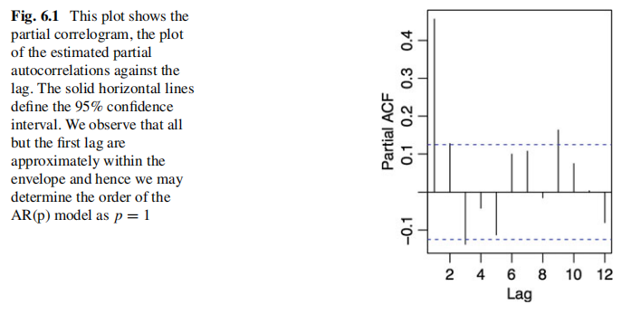
Partial Autocorrelations
- The order, , of a AR(p) model can be determined from time series data provided the data is stationary.
- This signature encodes the memory in the model and is given by "partial autocorrelations."
- each partial autocorrelation measures the correlation of a random variable, , with its lag, , while controlling for intermediate lags.
Partial Autocorrelation
A partial autocorrelation at lag is a conditional autocorrelation between a variable, , and its th lag, under the assumption that the values of the intermediate lags, are controlled:
where
is the lag- partial autocovariance, is an orthogonal projection of onto the set and
The partial autocorrelation function is a map . The plot of against is referred to as the partial correlogram.
Maximum Likelihood Estimation
-
The exact likelihood when the density of the data is independent of is
-
the exact likelihood is proportional to the conditional likelihood function:
-
In many cases such an assumption about the independence of the density of the data and the parameters is not warranted.
- the zero mean with unknown noise variance:
- The exact likelihood is
- the zero mean with unknown noise variance:
Heteroscedasticity
- heteroscedastic model
- the ARCH test: The ARCH Engle’s test is constructed based on the property that if the residuals are heteroscedastic, the squared residuals are autocorrelated. The Ljung–Box test is then applied to the squared residuals
- The estimation procedure for heteroscedastic models
- estimation of the errors from the maximum likelihood function which treats the errors as independent
- estimation of model parameters under a more general maximum likelihood estimation which treats the errors as time-dependent.
- The conditional likelihood is
where is the diagonal covariance matrix and is the data matrix defined as .
Moving Average Processes
- The Wold representation theorem (a.k.a. Wold decomposition): every covariance stationary time series can be written as the sum of two time series, one deterministic and one stochastic.
- the deterministic component: AR(p) process.
- the stochastic component: "moving average process" or process
Process
The th order moving average process is the linear combination of the white noise process
- an AR(1) process can be rewritten as a process.
- Suppose that the AR(1) process has a mean and the variance of the noise is , then by a binomial expansion of the operator we have
- where the moments can be easily found and are
- Suppose that the AR(1) process has a mean and the variance of the noise is , then by a binomial expansion of the operator we have
GARCH
- Generalized Autoregressive Conditional Heteroscedastic (GARCH) model
- parametric
- linear
- heteroscedastic
- GARCH(p,q) model specifies that the conditional variance (i.e., volatility) is given by an model-there are lagged conditional variances and lagged squared noise terms:
- A necessary condition for model stationarity is the following constraint:
- When the model is stationary, the long-run volatility converges to the unconditional variance of :
Exponential Smoothing
- the setting
- smoothing factor / smoothing coefficient:
- smoothed predictions:
- forecast error:
- the model
or equivalently
Fitting Time Series Models: The Box-Jenkins Approach
The three basic steps of the Box-Jenkins modeling approach:
- (I)dentification: determining the order of the model (a.k.a. model selection);
- (E)stimation: estimation of model parameters;
- (D)iagnostic checking: evaluating the fit of the model.
Stationarity
- Before the order of the model can be determined, the time series must be tested for stationarity.
- Augmented Dickey-Fuller (ADF) test
- A standard statistical test for covariance stationarity
- accounts for the (c)onstant drift and (t)ime trend
- Attempting to fit a time series model to non-stationary data will result in dubious interpretations of the estimated partial autocorrelation function and poor predictions and should therefore be avoided.
Transformation to Ensure Stationarity
- Any trending time series process is non-stationary.
- Detrending methods
- differencing
- Kalman filters
- Markov-switching models
- advanced neural networks
Identification
partial correlogram
Inforation Criterion
-
use the Akaike Information Criteria (AIC) to measure the quality of fit
- is the residual variance
- is the total number of parameters estimated.
-
The goal is to select the model which minimizes the AIC by first using maximum likelihood estimation and then adding the penalty term.
-
the AIC favors the best fit with the fewest number of parameters.
-
It is similar with regularization in machine learning where the loss function is penalized by a LASSO penalty norm of the parameters) or a ridge penalty ( norm of the parameters).
-
AIC is estimated post-hoc, once the maximum likelihood function is evaluated, whereas in machine learning models, the penalized loss function is directly minimized.
Model Diagnostics
- Once the model is fitted we must assess whether the residual exhibits autocorrelation, suggesting the model is underfitting.
- The residual of fitted time series model should be white noise.
A short summary of some of the most useful diagnostic tests for time series modeling in finance
| Name | Description |
|---|---|
| Chi-squared test | Used to determine whether the confusion matrix of a classifier is statistically significant, or merely white noise |
| t-test | Used to determine whether the output of two separate regression models are statistically different on i.i.d. data |
| Mariano-Diebold test | Used to determine whether the output of two separate time series models are statistically different |
| ARCH test | The ARCH Engle’s test is constructed based on the property that if the residuals are heteroscedastic, the squared residuals are autocorrelated. The Ljung–Box test is then applied to the squared residuals |
| Portmanteau test | A general test for whether the error in a time series model is auto-correlated Example tests include the Box-Ljung and the Box-Pierce test |
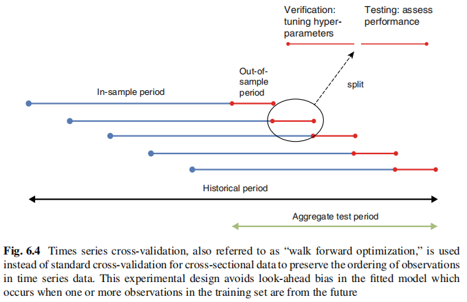
Time Series Cross-Validation
Summary
We have covered the following objectives:
- Explain and analyze linear autoregressive models;
- Understand the classical approaches to identifying, fitting, and diagnosing autoregressive models;
- Apply simple heteroscedastic regression techniques to time series data;
- Understand how exponential smoothing can be used to predict and filter time series