L05a Neural Networks for Structured Data

Materials are adopted from "Murphy, Kevin P. Probabilistic machine learning: an introduction. MIT press, 2022.". This handout is only for teaching. DO NOT DISTRIBUTE.

• L05a Neural Networks for Structured Data
  • Introduction
  • Multilayer perceptrons (MLPs)
    • The XOR problem
    • Differentiable MLPs
    • Activation functions (激活函数)
    • Example models
      • MLP for classifying $2 \mathrm{~d}$ data into 2 categories
      • MLP for image classification
      • MLP for text classification
      • MLP for heteroskedastic regression
    • The importance of depth
    • The "deep learning revolution"
    • Connections with biology
  • Backpropagation
    • Forward vs reverse mode differentiation
    • Computation graphs
  • Training neural networks
    • Tuning the learning rate
    • Vanishing and exploding gradients
    • Non-saturating activation functions
      • ReLU
      • Non-saturating ReLU
      • Other choices
    • Residual connections
  • Regularization
    • Early stopping
    • Weight decay
    • Dropout
    • Bayesian neural networks

Introduction

So far, we have learned：

• linear input-output mapping

  • logistic regression:
    • $p(y \mid x, w)=$ $\operatorname{Ber}\left(y \mid \sigma\left(w^{\top} \boldsymbol{x}\right)\right)$
    • multiclass case: $p(y \mid x, \mathbf{W})=\operatorname{Cat}(y \mid \mathcal{S}(\mathbf{W} \boldsymbol{x}))$
  • linear regression: $p(y \mid \boldsymbol{x}, \boldsymbol{w})=\mathcal{N}\left(y \mid \boldsymbol{w}^{\top} \boldsymbol{x}, \sigma^{2}\right)$
  • generalized linear models: Poisson dist. etc.

• models/algorithms linear in parameters

  • feature transformation, by replacing $x$ with $\phi(x)$
  • polynomial transform (in $1 \mathrm{~d}$): $\phi(x)=\left[1, x, x^{2}, x^{3}, \ldots\right]$
    $$f(\boldsymbol{x} ; \boldsymbol{\theta})=\mathbf{W} \phi(\boldsymbol{x})+\boldsymbol{b}$$

• deep neural networks or DNNs

  • to endow the feature extractor with its own parameters, $\theta_{2}$
    $$f(x ; \theta)=\mathbf{W} \phi\left(x ; \theta_{2}\right)+b$$
  • $\theta=\left(\theta_{1}, \theta_{2}\right)$ and $\theta_{1}=(\mathbf{W}, b)$
  • repeat this process recursively, to create more and more complex functions
    $$f(\boldsymbol{x} ; \boldsymbol{\theta})=f_{L}\left(f_{L-1}\left(\cdots\left(f_{1}(\boldsymbol{x})\right) \cdots\right)\right)$$
  • where $f_{\ell}(\boldsymbol{x})=f\left(\boldsymbol{x} ; \boldsymbol{\theta}_{\ell}\right)$ is the function at layer $\ell$

• The term "DNN" actually encompasses a larger family of models, in which we compose differentiable functions into any kind of DAG (directed acyclic graph, 有向无环图), mapping input to output.

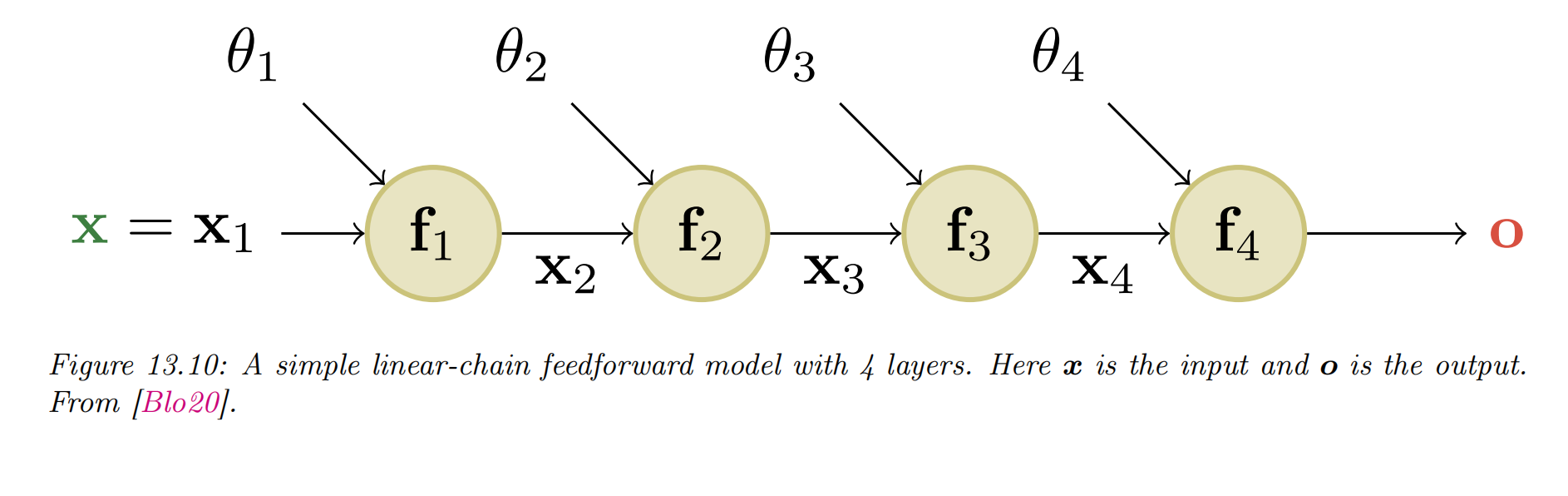
  • feedforward neural network (FFNN) or multilayer perceptron (MLP): the DAG is a chain.
  • A MLP is for "structured data" or "tabular data": $\boldsymbol{x} \in \mathbb{R}^{D}$
  • each column (feature) has a specific meaning

• DNNs for “unstructured data”

  • “unstructured data”: images, text
    • the input data is variable sized
    • each individual element (e.g., pixel or word) is often meaningless on its own
  • DNNs
    • convolutional neural networks (CNN) $\rightarrow$ images
    • recurrent neural networks (RNN) and transformers $\rightarrow$ sequences
    • graph neural networks (GNN) $\rightarrow$ graphs.

---

Multilayer perceptrons (MLPs)

• perceptron (感知机)
  • is a deterministic version of logistic regression
  • the functional form:
    $$f(\boldsymbol{x};\boldsymbol{\theta})=\mathbb{I}(\boldsymbol{w}^\top\boldsymbol{x}+b\geq0)=H(\boldsymbol{w}^\top\boldsymbol{x}+b)$$
  • $H(a)$: the heaviside step function, also known as a linear threshold function
  • perceptrons are very limited in what they can represent due to their linear decision boundaries

---

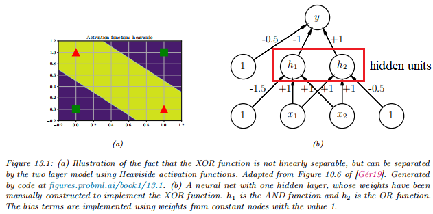
The XOR problem

• to learn a function that computes the exclusive OR （异-或逻辑） of its two binary inputs
• The truth table (真值表) for the function

$x_1$	$x_2$	$y$
0	0	0
0	1	1
1	0	1
1	1	0

• It is clear that the data is not linearly separable, so a perceptron cannot represent this mapping.

• this problem can be overcome by stacking multiple perceptrons on top of each other: multilayer perceptron (MLP)

• first hidden unit (AND operation) computes $h_1 = x_1 \wedge x_2$:

  • functional form:
    $$w^\top_1 x-b_1=[1.0,1.0]^\top[1,1]-1.5=0.5>0$$
  • $w_1$ are the weights
  • $b_1$ is the bias （偏置）
  • $h_1$ will fire iff $x_1$ and $x_2$ are both on

• the second hidden unit (OR operation) computes $h_{2}=x_{1} \vee x_{2}$

• the third unit computes the output $y=\overline{h_{1}} \wedge h_{2}$

  • where $\bar{h}=\neg h$ is the NOT (logical negation) operation
  • the $y$ value
    $$y=f\left(x_{1}, x_{2}\right)=\overline{\left(x_{1} \wedge x_{2}\right)} \wedge\left(x_{1} \vee x_{2}\right)$$

• This is equivalent to the XOR function

An MLP can represent any logical function. However, we obviously want to avoid having to specify the weights and biases by hand. In the rest of this chapter, we discuss ways to learn these parameters from data.

---

Differentiable MLPs

• MLPs are difficult to train
  • the heaviside function is non-differentiable
• A natural solution: replacing the heaviside function with a differeentiable one (i.e. the activation function $\varphi: \mathbb{R} \rightarrow \mathbb{R}$)
• the big idea:

  • define the hidden units $z_{l}$ at each layer $l$ to be a linear transformation of the hidden units at the previous layer passed elementwise through this activation function

    • functional form
      $$z_{l}=f_{l}\left(z_{l-1}\right)=\varphi_{l}\left(b_{l}+\mathbf{W}_{l} z_{l-1}\right)$$
    • in scalar form,
      $$z_{k l}=\varphi_{l}\left(b_{k l}+\sum_{j=1}^{K_{l-1}} w_{j k l} z_{j l-1}\right)$$

  • pre-activations: The quantity that is passed to the activation function
    $$a_{l}=b_{l}+\mathbf{W}_{l} z_{l-1}$$

    • $z_{l}=\varphi_{l}\left(a_{l}\right)$.

  • backpropagation (反向传播算法):

    • compose $L$ of these functions together
    • compute the gradient of the output wrt the parameters in each layer using the chain rule
    • pass the gradient to an optimizer to minimize some training objective

---

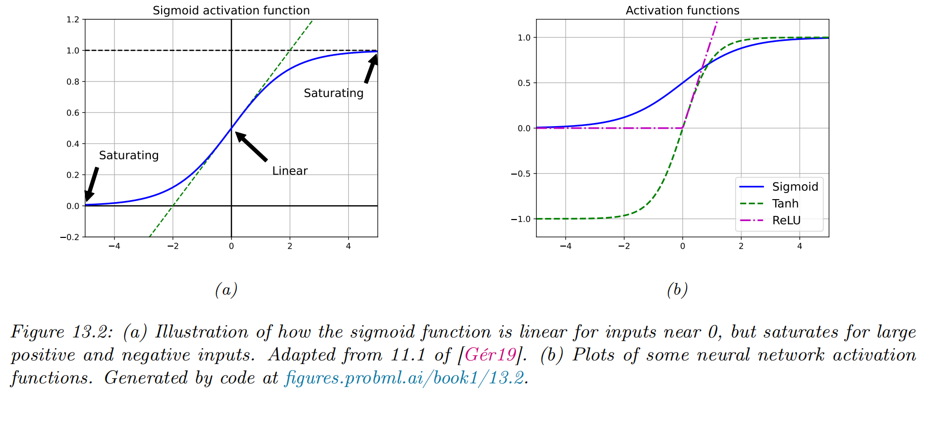
Activation functions (激活函数)

• linear activation function, $\varphi_{\ell}(a)=c_{\ell} a$, makes the whole model reduces to a regular linear model
  $$f(\boldsymbol{x} ; \boldsymbol{\theta})=\mathbf{W}_{L} c_{L}\left(\mathbf{W}_{L-1} c_{L-1}\left(\cdots\left(\mathbf{W}_{1} \boldsymbol{x}\right) \cdots\right)\right) \propto \mathbf{W}_{L} \mathbf{W}_{L-1} \cdots \mathbf{W}_{1} \boldsymbol{x}=\mathbf{W}^{\prime} \boldsymbol{x}$$

• nonlinear activation functions.

  • sigmoid (logistic) function
    • a smooth approximation to the Heaviside function used in a perceptron:
      $$\boldsymbol{\sigma}(a)=\frac{1}{1+e^{-a}}$$
    • it saturates(饱和) at 1 for large positive inputs, and at 0 for large negative inputs
      
    • 因为Logistic函数的性质，使得装备了Logistic激活函数的神经元具有以下两点性质：
      • 其输出直接可以看作是概率分布，使得神经网络可以更好地和统计学习模型进行结合。
      • 其可以看作是一个软性门（Soft Gate），用来控制其它神经元输出信息的数量。
  • the tanh function（双曲正切函数）
    $$\tanh(x)=\frac{\exp(x)-\exp(-x)}{\exp(x)+\exp(-x)}$$
    • Tanh 函数可以看作是放大并平移的 Logistic 函数，其值域是 $( − 1, 1)$。
      $$\tanh(x)=2\sigma(2x)-1$$
    • has a similar shape
    • saturates at $-1$ and $+1$
    • Tanh 函数的输出是零中心化的（Zero-Centered），而 Logistic 函数的输出恒大于 0。非零中心化的输出会使得其后一层的神经元的输入发生偏置偏移（Bias Shift），并进一步使得梯度下降的收敛速度变慢。
  • vanishing gradient problem
    • the gradient of the output wrt the input will be close to zero
    • any gradient signal from higher layers will not be able to propagate back to earlier layers
    • it makes it hard to train the model using gradient descent
  • rectified linear unit（修正线性单元） or ReLU
    • a non-saturating activation functions
    • make it possible to train very deep models
    • it "turns off" negative inputs, and passes positive inputs unchanged
      $$\operatorname{ReLU}(a)=\max (a, 0)=a \mathbb{I}(a>0)$$

---

Example models

MLPs can be used to perform classification and regression for many kinds of data. We give some examples below.

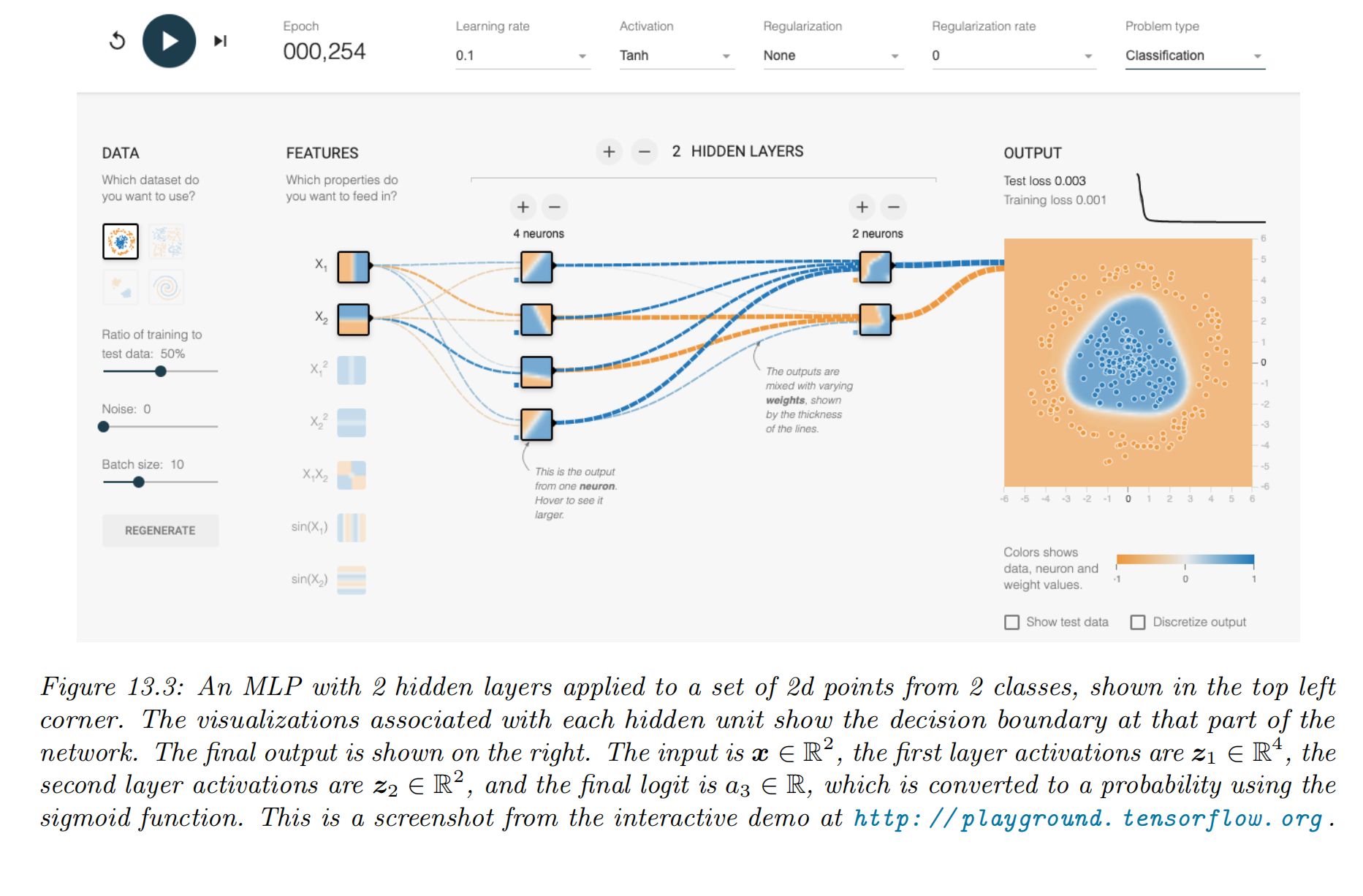
Try it for yourself via: https://playground.tensorflow.org

MLP for classifying $2 \mathrm{~d}$ data into 2 categories

an MLP with two hidden layers applied to a 2 d input vector (Figure $13.3$)

• the model:
  $$\begin{aligned} p(y \mid \boldsymbol{x} ; \boldsymbol{\theta}) &=\operatorname{Ber}\left(y \mid \boldsymbol{\sigma}\left(a_{3}\right)\right) \\ a_{3} &=\boldsymbol{w}_{3}^{\top} \boldsymbol{z}_{2}+b_{3} \\ \boldsymbol{z}_{2} &=\varphi\left(\mathbf{W}_{2} \boldsymbol{z}_{1}+\boldsymbol{b}_{2}\right) \\ \boldsymbol{z}_{1} &=\varphi\left(\mathbf{W}_{1} \boldsymbol{x}+\boldsymbol{b}_{1}\right) \end{aligned}$$
• $a_{3}=\boldsymbol{w}_{3}^{\top} z_{2}+b_{3}$ is the final logit score, which is converted to a probability via the sigmoid (logistic) function.
• layer 2 is computed by taking a nonlinear combination of the 4 hidden units in layer 1 , using $z_{2}=\varphi\left(\mathbf{W}_{2} \boldsymbol{z}_{1}+\boldsymbol{b}_{2}\right)$
• layer 1 is computed by taking a nonlinear combination of the 2 input units, using $\boldsymbol{z}_{1}=\varphi\left(\mathbf{W}_{1} \boldsymbol{x}+\boldsymbol{b}_{1}\right)$
• By adjusting the parameters, $\boldsymbol{\theta}=\left(\mathbf{W}_{1}, \boldsymbol{b}_{1}, \mathbf{W}_{2}, \boldsymbol{b}_{2}, \boldsymbol{w}_{3}, b_{3}\right)$, to minimize the negative log likelihood, we can fit the training data very well

MLP for image classification

• "flatten" the 2 d input into 1 d vector: $28 \times 28=784$ dimensional
• NN structure: use 2 hidden layers with 128 units each, followed by a final 10 way softmax layer

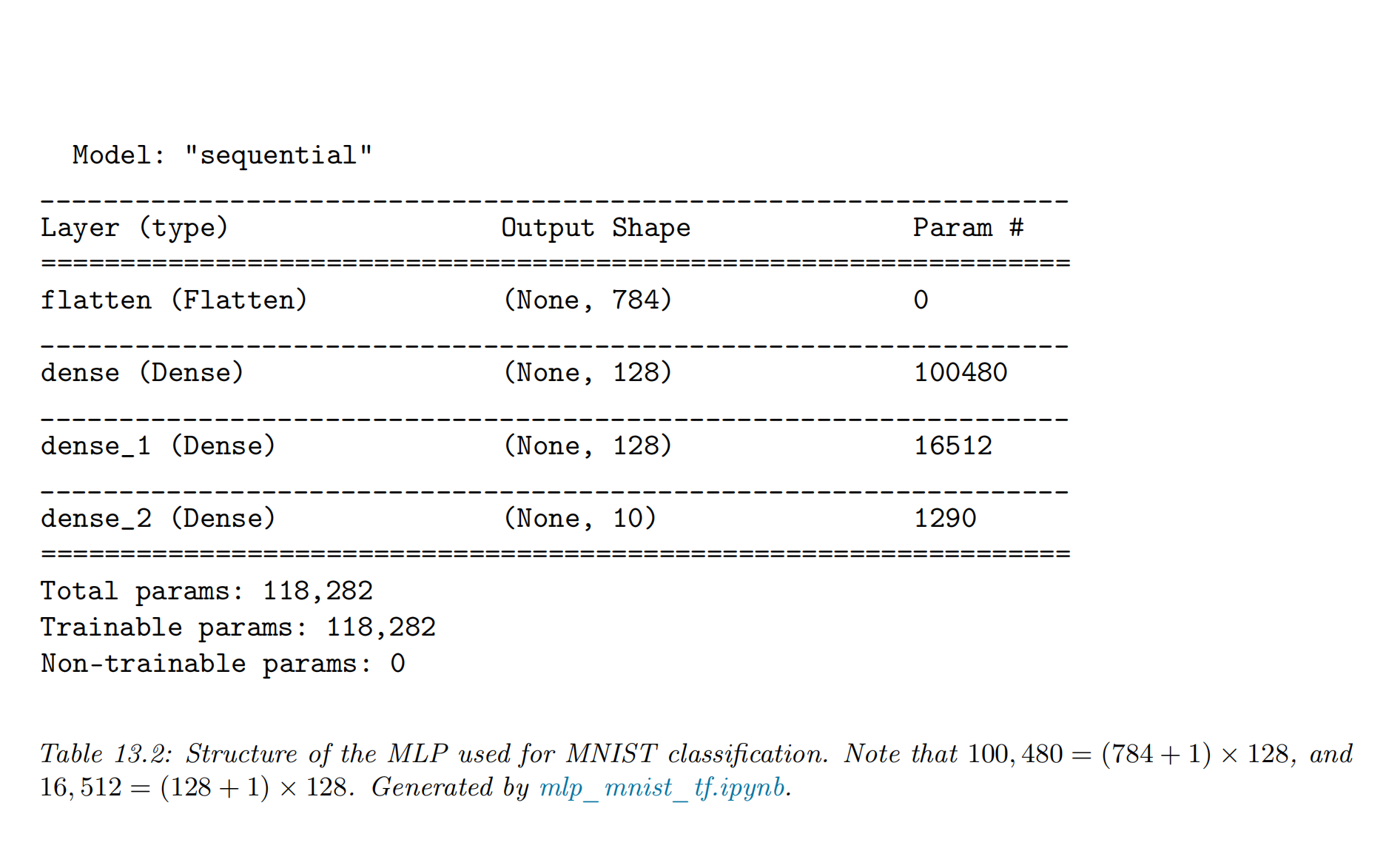
• training results
  • train for just two "epochs" (passes over the dataset)
  • test set accuracy of $97.1 \%$
  • the errors seem sensible, e.g., 9 is mistaken as a 3
  • Training for more epochs can further improve test accuracy

MLP for text classification

• convert the variable-length sequence of words $\boldsymbol{v}_{1}, \ldots, \boldsymbol{v}_{T}$ into a fixed dimensional vector $\boldsymbol{x}$
  • each $\boldsymbol{v}_{t}$ is a one-hot vector of length $V$
  • $V$ is the vocabulary size
• the method
  • treat the input as an unordered bag of words $\left\{\boldsymbol{v}_{t}\right\}$
  • the first layer of the model is a $E \times V$ embedding matrix $\mathbf{W}_{1}$, which converts each sparse $V$-dimensional vector to a dense $E$-dimensional embedding, $\boldsymbol{e}_{t}=\mathbf{W}_{1} \boldsymbol{v}_{t}$
  • convert this set of $TE$-dimensional embeddings into a fixed-sized vector using global average pooling, $\bar{e}=\frac{1}{T} \sum_{t=1}^{T} e_{t}$
• example:
  • a single hidden layer
  • a logistic output (for binary classification), we get
    $$\begin{aligned} p(y \mid \boldsymbol{x} ; \boldsymbol{\theta}) &=\operatorname{Ber}\left(y \mid \boldsymbol{\sigma}\left(\boldsymbol{w}_{3}^{\top} \boldsymbol{h}+b_{3}\right)\right) \\ \boldsymbol{h} &=\varphi\left(\mathbf{W}_{2} \overline{\boldsymbol{e}}+\boldsymbol{b}_{2}\right) \\ \overline{\boldsymbol{e}} &=\frac{1}{T} \sum_{t=1}^{T} \boldsymbol{e}_{t} \\ \boldsymbol{e}_{t} &=\mathbf{W}_{1} \boldsymbol{v}_{t} \end{aligned}$$

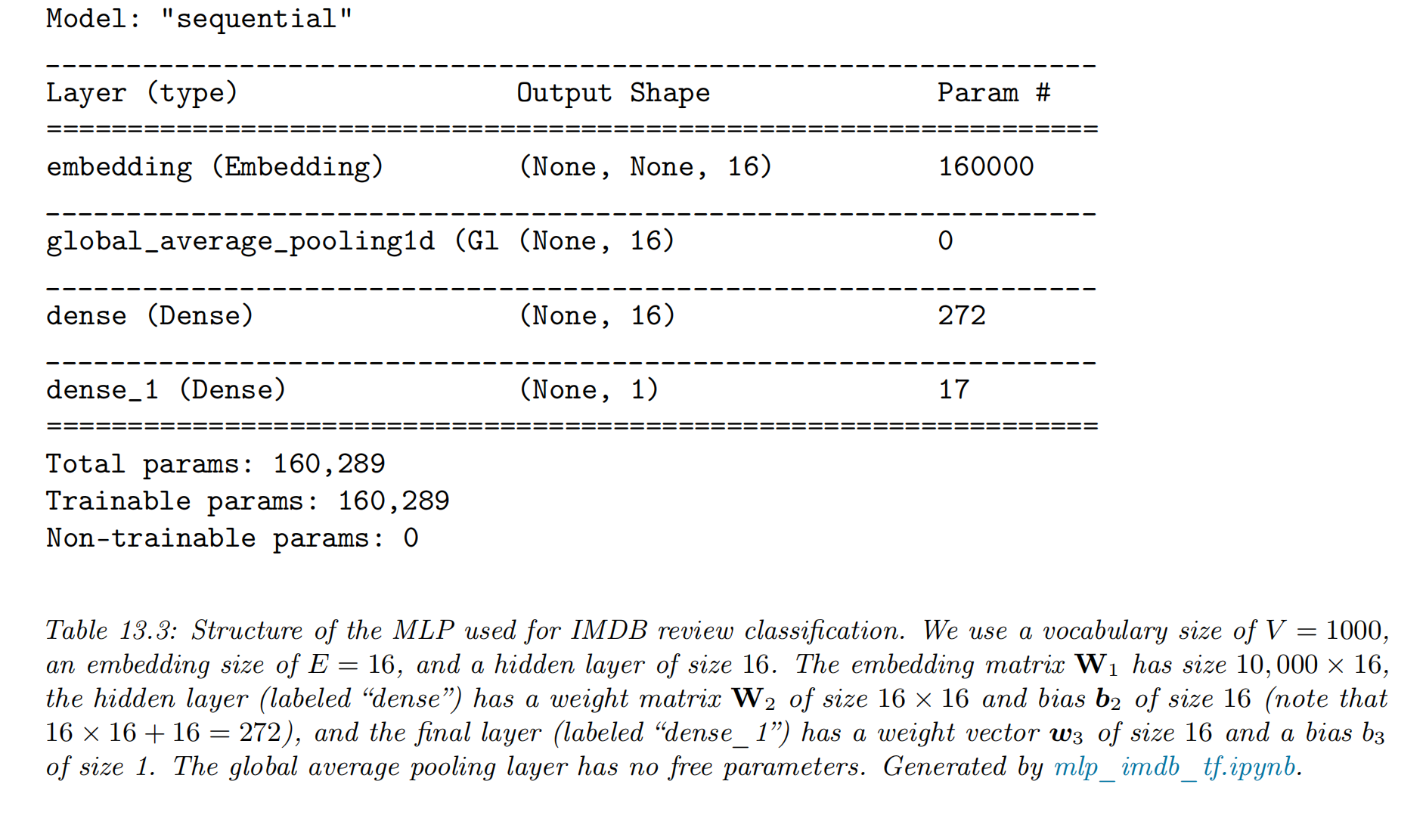
• NN setting & the training result
  • vocabulary size: $V=1000$
  • embedding size of $E=16$
  • hidden layer of size 16
  • we get $86 \%$ on the validation set.

MLP for heteroskedastic regression

• a model for heteroskedastic nonlinear regression
• outputs:
  • $f_{\mu}(\boldsymbol{x})=\mathbb{E}[y \mid \boldsymbol{x}, \boldsymbol{\theta}]$
  • $f_{\sigma}(\boldsymbol{x})=\sqrt{\mathbb{V}[y \mid \boldsymbol{x}, \boldsymbol{\theta}]}$.
• The two heads:
  • the $\mu$ head, we use a linear activation, $\varphi(a)=a$
  • the $\sigma$ head, we use a softplus activation, $\varphi(a)=\sigma_{+}(a)=\log \left(1+e^{a}\right)$.
• linear heads and a nonlinear backbone, the overall model is given by
  $$p(y \mid \boldsymbol{x}, \boldsymbol{\theta})=\mathcal{N}\left(y \mid \boldsymbol{w}_{\boldsymbol{\mu}}^{\top} f\left(\boldsymbol{x} ; \boldsymbol{w}_{\text {shared }}\right), \sigma_{+}\left(\boldsymbol{w}_{\boldsymbol{\sigma}}^{\top} f\left(\boldsymbol{x} ; \boldsymbol{w}_{\text {shared }}\right)\right)\right)$$

• stochastic volatility model
  • properties
    • the mean grows linearly over time
    • seasonal oscillations
    • the variance increases quadratically
  • applications
    • financial data
    • global temperature of the earth

---

The importance of depth

• an MLP with one hidden layer is a universal function approximator

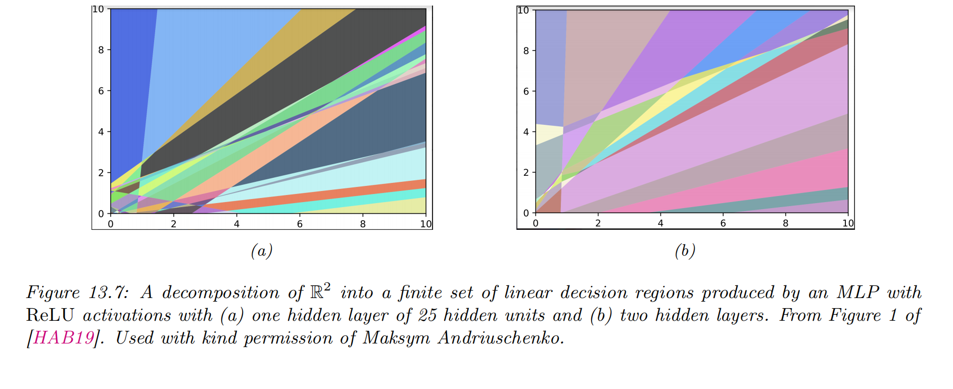
• deep networks work better than shallow ones
• the benefit of learning via a compositional or hierarchical way
• Example:
  • classify DNA strings
  • the positive class is associated with the regular expression AA??CGCG??AA
  • it will be easier to learn if the model first learns to detect the AA and CG “motifs” using the hidden units in layer 1
  • then uses these features to define a simple linear classifier in layer 2

---

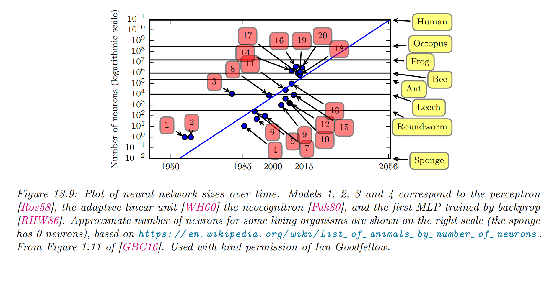
The "deep learning revolution"

• some successful stories about DNNs
  • automatic speech recognition (ASR)
  • ImageNet image classification benchmark: reducing the error rate from 26% to 16% in a single year
• The “explosion” in the usage of DNNs
  • the availability of cheap GPUs (graphics processing units)
  • the growth in large labeled datasets
• high quality open-source software libraries for DNNs
  • Tensorflow (made by Google)
  • PyTorch (made by Facebook)
  • MXNet (made by Amazon)
  • PaddlePaddle 飞桨 （百度）

---

Connections with biology

• McCulloch-Pitts model of the neuron (1943): $h_k(\boldsymbol{x}) = H(w^\top_kx − b_k)$, where $H(a) = \mathbb{I}(a > 0)$

  • the inputs $\boldsymbol{x} \in\mathbb{R}^D$
  • the strength of the incoming connections $\boldsymbol{w}_k \in\mathbb{R}^D$
  • weighted (dendrites树突) sum of the inputs $a_k = w^\top_kx$
  • threshold (action potential动作电位) $b_k$
  • $h_k=1\rightarrow\text{fire}$

• We can combine multiple such neurons together to make an artificial neural networks, ANNs

• ANNs differs from biological brains in many ways, including the following:

• Most ANNs use backpropagation to modify the strength of their connections while real brains do not use backprop

  • there is no way to send information backwards along an axon
  • they use local update rules for adjusting synaptic strengths

• Most ANNs are strictly feedforward (前馈的), but real brains have many feedback connections

  • It is believed that this feedback acts like a prior

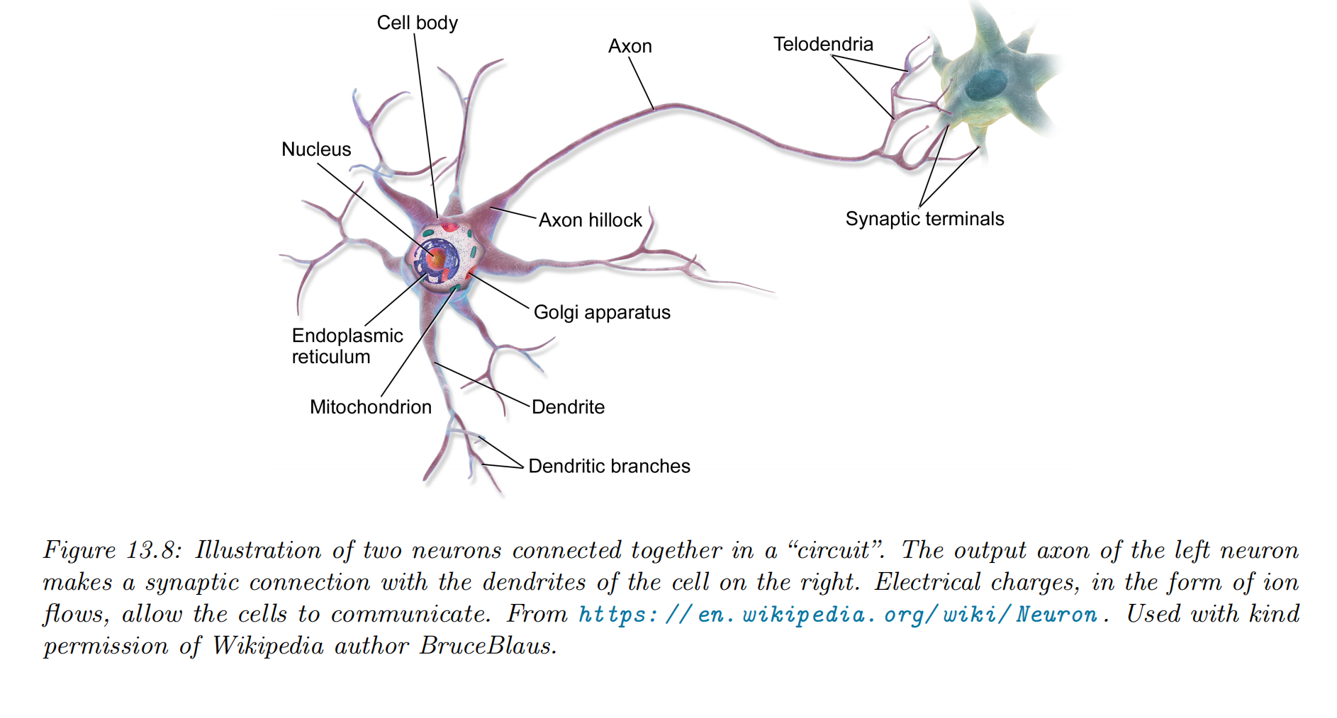
• Most ANNs use simplified neurons consisting of a weighted sum passed through a nonlinearity, but real biological neurons have complex dendritic tree structures (see Figure 13.8), with complex spatio-temporal dynamics.

• Most ANNs are smaller in size and number of connections than biological brains

• Most ANNs are designed to model a single function while biological brains are very complex systems that implement different kinds of functions or behaviors

---

Backpropagation

• backpropagation
  • simple linear chain of stacked layers: repeated applications of the chain rule of calculus
  • arbitrary directed acyclic graphs (DAGs): automatic differentiation or autodiff.

---

Forward vs reverse mode differentiation

• Consider a mapping of the form $\boldsymbol{o}=\boldsymbol{f}(\boldsymbol{x})$

  • $\boldsymbol{x} \in \mathbb{R}^{n}$ and $\boldsymbol{o} \in \mathbb{R}^{m}$
  • $\boldsymbol{f}$ is defined as a composition of functions:
    $$f=f_{4} \circ f_{3} \circ f_{2} \circ f_{1}$$
  • $\boldsymbol{f}_{1}: \mathbb{R}^{n} \rightarrow \mathbb{R}^{m_{1}}, \boldsymbol{f}_{2}: \mathbb{R}^{m_{1}} \rightarrow \mathbb{R}^{m_{2}}, \boldsymbol{f}_{3}: \mathbb{R}^{m_{2}} \rightarrow \mathbb{R}^{m_{3}}$, and $\boldsymbol{f}_{4}: \mathbb{R}^{m_{3}} \rightarrow \mathbb{R}^{m}$
  • The intermediate steps needed to compute $\boldsymbol{o}=\boldsymbol{f}(\boldsymbol{x})$ are $\boldsymbol{x}_{2}=\boldsymbol{f}_{1}(\boldsymbol{x}), \boldsymbol{x}_{3}=\boldsymbol{f}_{2}\left(\boldsymbol{x}_{2}\right), \boldsymbol{x}_{4}=\boldsymbol{f}_{3}\left(\boldsymbol{x}_{3}\right)$, and $\boldsymbol{o}=\boldsymbol{f}_{4}\left(\boldsymbol{x}_{4}\right)$.

• We can compute the Jacobian $\mathbf{J}_{\boldsymbol{f}}(\boldsymbol{x})=\frac{\partial \boldsymbol{o}}{\partial \boldsymbol{x}^{\top}} \in \mathbb{R}^{m \times n}$ using the chain rule:
  $$\begin{aligned} \frac{\partial \boldsymbol{o}}{\partial \boldsymbol{x}} &=\frac{\partial \boldsymbol{o}}{\partial \boldsymbol{x}_{4}} \frac{\partial \boldsymbol{x}_{4}}{\partial \boldsymbol{x}_{3}} \frac{\partial \boldsymbol{x}_{3}}{\partial \boldsymbol{x}_{2}} \frac{\partial \boldsymbol{x}_{2}}{\partial \boldsymbol{x}}=\frac{\partial \boldsymbol{f}_{4}\left(\boldsymbol{x}_{4}\right)}{\partial \boldsymbol{x}_{4}} \frac{\partial \boldsymbol{f}_{3}\left(\boldsymbol{x}_{3}\right)}{\partial \boldsymbol{x}_{3}} \frac{\partial \boldsymbol{f}_{2}\left(\boldsymbol{x}_{2}\right)}{\partial \boldsymbol{x}_{2}} \frac{\partial \boldsymbol{f}_{1}(\boldsymbol{x})}{\partial \boldsymbol{x}} \\ &=\mathbf{J}_{\boldsymbol{f}_{4}}\left(\boldsymbol{x}_{4}\right) \mathbf{J}_{\boldsymbol{f}_{3}}\left(\boldsymbol{x}_{3}\right) \mathbf{J}_{\boldsymbol{f}_{2}}\left(\boldsymbol{x}_{2}\right) \mathbf{J}_{\boldsymbol{f}_{1}}(\boldsymbol{x}) \end{aligned}$$

• we only need to consider how to compute the Jacobian efficiently

---

Computation graphs

• Modern DNNs can combine differentiable components in much more complex ways, to create a computation graph, analogous to how programmers combine elementary functions to make more complex ones.

• The only restriction is that the resulting computation graph corresponds to a directed ayclic graph (DAG), where each node is a differentiable function of all its inputs.

• example
  $$f\left(x_{1}, x_{2}\right)=x_{2} e^{x_{1}} \sqrt{x_{1}+x_{2} e^{x_{1}}}$$

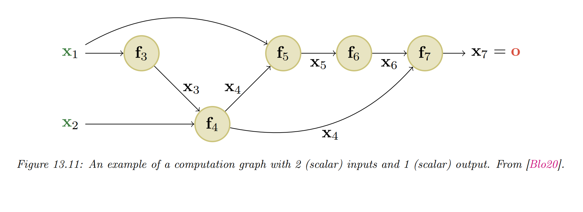
• We can compute this using the DAG in Figure 13.11, with the following intermediate functions:
  $$\begin{aligned} &x_{3}=f_{3}\left(x_{1}\right)=e^{x_{1}} \\ &x_{4}=f_{4}\left(x_{2}, x_{3}\right)=x_{2} x_{3} \\ &x_{5}=f_{5}\left(x_{1}, x_{4}\right)=x_{1}+x_{4} \\ &x_{6}=f_{6}\left(x_{5}\right)=\sqrt{x_{5}} \\ &x_{7}=f_{7}\left(x_{4}, x_{6}\right)=x_{4} x_{6} \end{aligned}$$
  • we have numbered the nodes in topological order (parents before children)
  • During the backward pass, since the graph is no longer a chain, we may need to sum gradients along multiple paths. For example, since $x_{4}$ influences $x_{5}$ and $x_{7}$, we have
    $$\frac{\partial \boldsymbol{o}}{\partial \boldsymbol{x}_{4}}=\frac{\partial \boldsymbol{o}}{\partial \boldsymbol{x}_{5}} \frac{\partial \boldsymbol{x}_{5}}{\partial \boldsymbol{x}_{4}}+\frac{\partial \boldsymbol{o}}{\partial \boldsymbol{x}_{7}} \frac{\partial \boldsymbol{x}_{7}}{\partial \boldsymbol{x}_{4}}$$
  • We can avoid repeated computation by working in reverse topological order. For example,
    $$\begin{aligned} \frac{\partial \boldsymbol{o}}{\partial \boldsymbol{x}_{7}} &=\frac{\partial \boldsymbol{x}_{7}}{\partial \boldsymbol{x}_{7}}=\mathbf{I}_{m} \\ \frac{\partial \boldsymbol{o}}{\partial \boldsymbol{x}_{6}} &=\frac{\partial \boldsymbol{o}}{\partial \boldsymbol{x}_{7}} \frac{\partial \boldsymbol{x}_{7}}{\partial \boldsymbol{x}_{6}} \\ \frac{\partial \boldsymbol{o}}{\partial \boldsymbol{x}_{5}} &=\frac{\partial \boldsymbol{o}}{\partial \boldsymbol{x}_{6}} \frac{\partial \boldsymbol{x}_{6}}{\partial \boldsymbol{x}_{5}} \\ \frac{\partial \boldsymbol{o}}{\partial \boldsymbol{x}_{4}} &=\frac{\partial \boldsymbol{o}}{\partial \boldsymbol{x}_{5}} \frac{\partial \boldsymbol{x}_{5}}{\partial \boldsymbol{x}_{4}}+\frac{\partial \boldsymbol{o}}{\partial \boldsymbol{x}_{7}} \frac{\partial \boldsymbol{x}_{7}}{\partial \boldsymbol{x}_{4}} \end{aligned}$$
  • In general, we use
    $$\frac{\partial \boldsymbol{o}}{\partial \boldsymbol{x}_{j}}=\sum_{k \in \operatorname{children}(j)} \frac{\partial \boldsymbol{o}}{\partial \boldsymbol{x}_{k}} \frac{\partial \boldsymbol{x}_{k}}{\partial \boldsymbol{x}_{j}}$$

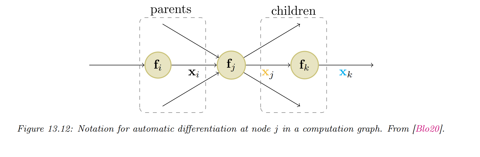
where the sum is over all children $k$ of node $j$, as shown in Figure $13.12$. The $\frac{\partial \boldsymbol{o}}{\partial \boldsymbol{x}_{k}}$ gradient vector has already been computed for each child $k$; this quantity is called the adjoint. This gets multiplied by the Jacobian $\frac{\partial \boldsymbol{x}_{k}}{\partial \boldsymbol{x}_{j}}$ of each child.

---

Training neural networks

• fit DNNs to data
• The standard approach is to use maximum likelihood estimation, by minimizing the NLL:
  $$\mathcal{L}(\boldsymbol{\theta})=-\log p(\mathcal{D} \mid \boldsymbol{\theta})=-\sum_{n=1}^{N} \log p\left(\boldsymbol{y}_{n} \mid \boldsymbol{x}_{n} ; \boldsymbol{\theta}\right)$$

---

Tuning the learning rate

It is important to tune the learning rate (step size), to ensure convergence to a good solution. (Section 8.4.3.)

---

Vanishing and exploding gradients

• vanishing gradient problem（梯度消失）: When training very deep models, the gradient become very small

• exploding gradient problem（梯度爆炸）: When training very deep models, the gradient become very large

• consider the gradient of the loss wrt a node at layer $l$ :
  $$\frac{\partial \mathcal{L}}{\partial \boldsymbol{z}_{l}}=\frac{\partial \mathcal{L}}{\partial \boldsymbol{z}_{l+1}} \frac{\partial \boldsymbol{z}_{l+1}}{\partial \boldsymbol{z}_{l}}=\mathbf{J}_{l} \boldsymbol{g}_{l+1}$$

  • $\mathbf{J}_{l}=\frac{\partial \boldsymbol{z}_{l+1}}{\partial \boldsymbol{z}_{l}}$ is the Jacobian matrix
  • $\boldsymbol{g}_{l+1}=\frac{\partial \mathcal{L}}{\partial \boldsymbol{z}_{l+1}}$ is the gradient at the next layer. If $\mathbf{J}_{l}$ is constant across layers, it is clear that the contribution of the gradient from the final layer, $\boldsymbol{g}_{L}$, to layer $l$ will be $\mathbf{J}^{L-l} \boldsymbol{g}_{L}$. Thus the behavior of the system depends on the eigenvectors of $\mathbf{J}$.

• The exploding gradient problem can be ameliorated by gradient clipping(梯度裁剪), in which we cap the magnitude of the gradient if it becomes too large, i.e., we use
  $$\boldsymbol{g}^{\prime}=\min \left(1, \frac{c}{\|\boldsymbol{g}\|}\right) \boldsymbol{g}$$

  • This way, the norm of $\boldsymbol{g}^{\prime}$ can never exceed $c$, but the vector is always in the same direction as $\boldsymbol{g}$.

• the vanishing gradient problem is more difficult to solve

  • Modify the the activation functions at each layer to prevent the gradient from becoming too large or too small
  • Modify the architecture so that the updates are additive rather than multiplicative
  • Modify the architecture to standardize the activations at each layer, so that the distribution of activations over the dataset remains constant during training
  • Carefully choose the initial values of the parameters

---

Non-saturating activation functions

reason for the gradient vanishe problem

• setting: $z=\sigma(\mathbf{W} x)$, where
  $$\varphi(a)=\sigma(a)=\frac{1}{1+\exp (-a)}$$

• for saturating activation functions
  $$\text{large weights}\rightarrow\boldsymbol{a}=\mathbf{W} \boldsymbol{x}\text{ large}\rightarrow\boldsymbol{z}\text{ to saturate}$$

• the gradient of the loss wrt the inputs $\boldsymbol{x}$ (from an earlier layer)
  $$\varphi^{\prime}(a)=\boldsymbol{\sigma}(a)(1-\sigma(a))$$

• the gradient of the loss wrt the inputs is
  $$\frac{\partial \mathcal{L}}{\partial \boldsymbol{x}}=\mathbf{W}^{\top} \boldsymbol{\delta}=\mathbf{W}^{\top} \boldsymbol{z}(1-\boldsymbol{z})$$

• the gradient of the loss wrt the parameters is
  $$\frac{\partial \mathcal{L}}{\partial \mathbf{W}}=\boldsymbol{\delta} \boldsymbol{x}^{\top}=\boldsymbol{z}(1-\boldsymbol{z}) \boldsymbol{x}^{\top}$$

• if $z$ is near 0 or 1 , the gradients will go to 0 .

• One of the keys to being able to train very deep models is to use non-saturating activation functions.

• Several different functions have been proposed: see Table $13.4$ for a summary, and https://mlfromscratch.com/activation-functions-explained for more details.

Name	Definition	Range	Reference
Sigmoid	$\sigma(a)=\frac{1}{1+e^{-a}}$	$[0,1]$
Hyperbolic tangent	$\tanh(a)=2\sigma(2a)-1$	$[-1,1]$
Softplus	$\sigma_+(a)=\log(1+e^2)$	$[0,\infty]$	[GBB11]
Rectified linear unit	$\operatorname{ReLU}(a) = \max(a, 0)$	$[0,\infty]$	[GBB11;KSH12]
Leaky ReLU	$\max(a, 0) + \alpha \min(a, 0)$	$[-\infty,\infty]$	[MHN13]
Exponential linear unit	$\max(a,0)+\min(\alpha(e^a-1),0)$	$[-\infty,\infty]$	[CUH16]
Swish	$a\sigma(a)$	$[-\infty,\infty]$	[RZL17]
GELU	$a\Phi(a)$	$[-\infty,\infty]$	[HG16]

ReLU

• The most common is rectified linear unit （修正线性单元） or ReLU
  $$\operatorname{ReLU}(a)=\max (a, 0)=a \mathbb{I}(a>0)$$
• The gradient has the following form:
  $$\operatorname{ReLU}^{\prime}(a)=\mathbb{I}(a>0)$$
• the gradient will not vanish, as long a $\boldsymbol{z}$ is positive.
  • suppose we use this in a layer to compute $\boldsymbol{z}=\operatorname{ReLU}(\mathbf{W} \boldsymbol{x})$.
  • the gradient wrt the inputs has the form
    $$\frac{\partial \mathcal{L}}{\partial \boldsymbol{x}}=\mathbf{W}^{\top} \mathbb{I}(\boldsymbol{z}>\mathbf{0})$$
• the gradient wrt the parameters
  $$\frac{\partial \mathcal{L}}{\partial \mathbf{W}}=\mathbb{I}(z>0) \boldsymbol{x}^{\top}$$
• the “dead ReLU” problem:
  • if the weights are initialized to be large and negative, then it becomes very easy for (some components of) $\boldsymbol{a}=\mathbf{W} \boldsymbol{x}$ to take on large negative values, and hence for $\boldsymbol{z}$ to go to 0 .
  • This will cause the gradient for the weights to go to 0 .
  • The algorithm will never be able to escape this situation,
  • the hidden units (components of $\boldsymbol{z}$) will stay permanently off.

Non-saturating ReLU

• the leaky ReLU
  $$\operatorname{LReLU}(a ; \alpha)=\max (\alpha a, a)$$

  • $0<\alpha<1$.
  • The slope of this function is 1 for positive inputs, and $\alpha$ for negative inputs, thus ensuring there is some signal passed back to earlier layers, even when the input is negative.
  • If we allow the parameter $\alpha$ to be learned, rather than fixed, the leaky ReLU is called parametric ReLU

• the Exponential Linear Unit, ELU (指数线性单元)
  $$\operatorname{ELU}(a ; \alpha)= \begin{cases}\alpha\left(e^{a}-1\right) & \text { if } a \leq 0 \\ a & \text { if } a>0\end{cases}$$

  • This has the advantage over leaky ReLU of being a smooth function.

• SELU (self-normalizing ELU): A slight variant of ELU
  $$\operatorname{SELU}(a ; \alpha, \lambda)=\lambda \operatorname{ELU}(a ; \alpha)$$

  • by setting $\alpha$ and $\lambda$ to carefully chosen values, this activation function is guaranteed to ensure that the output of each layer is standardized (provided the input is also standardized)
  • This can help with model fitting.

• Softplus函数[Dugas et al., 2001] 可以看作是 rectifier 函数的平滑版本，其定义为:

$$\text{Softplus}(x)=\log(1+\exp(x))$$

$$\text{Softplus}'(x)=\sigma(x)$$

Other choices

• swish (do well on some image classification benchmarks)
  $$\operatorname{swish}(a ; \beta)=a \sigma(\beta a)$$

  • also called SiLU (for Sigmoid Linear Unit)
  • $\sigma(\cdot)\in(0,1)$ 可看作一种软性门控机制：
    • $\sigma(\beta x)$接近1时，门处于“开”状态，激活函数的输出近似于 $x$ 本身
    • $\sigma(\beta x)$接近0时，门处于“关”状态，激活函数的输出近似于0

• Maxout单元
  Maxout 单元 [Goodfellow et al., 2013] 也是一种分段线性函数。其他激活函数输入为上一层神经元的尽输入$z$，Maxout的输入为上一层神经元的全部原始输入$x=[x_1,x_2,\dots,x_d]$。每个Maxout单元有$K$个权向量$w_k\in\mathbb{R}^d$和偏置$b_k (1\leq k\leq K)$:
  $$z_k=w_k^Tx+b_k$$
  Maxout单元非线性函数定义为：

$$\text{maxout}(x)=\max_{k\in[1,K]}(z_k)$$

• Gaussian Error Linear Unit, GELU
  $$\mathrm{GELU}(a)=a \Phi(a)$$
  • where $\Phi(a)$ is the cdf of a standard normal:
    $$\Phi(a)=\operatorname{Pr}(\mathcal{N}(0,1) \leq a)=\frac{1}{2}(1+\operatorname{erf}(a / \sqrt{2}))$$
  • We can think of GELU as a "soft" version of ReLU, since it replaces the step function $\mathbb{I}(a>0)$ with the Gaussian cdf, $\Phi(a)$.
  • the GELU can be motivated as an aptive version of dropout, where we multiply the input by a binary scalar mask, $m \sim \operatorname{Ber}(\Phi(a)$ ), where the probability of being dropped is given by $1-\Phi(a)$. Thus the expected output is
    $$\mathbb{E}[a]=\Phi(a) \times a+(1-\Phi(a)) \times 0=a \Phi(a)$$
  • We can approximate GELU using swish with a particular parameter setting, namely
    $$\operatorname{GELU}(a) \approx a \sigma(1.702 a)$$

---

Residual connections

• residual network or ResNet (残差网络)
  • One solution to the vanishing gradient problem for DNNs
  • this is a feedforward model in which each layer has the form of a residual block, defined by
    $$\mathcal{F}_{l}^{\prime}(x)=\mathcal{F}_{l}(x)+x$$
    • $\mathcal{F}_{l}$ is a standard shallow nonlinear mapping (e.g., linear-activation-linear).
    • The inner $\mathcal{F}_{l}$ function computes the residual term or delta that needs to be added to the input $x$ to generate the desired output
    • it is often easier to learn to generate a small perturbation to the input than to directly predict the output.

• A model with residual connections has the same number of parameters as a model without residual connections, but it is easier to train
  • gradients can flow directly from the output to earlier layers (Figure 13.15b)
  • the activations at the output layer can be derived in terms of any previous layer $l$ using
    $$z_{L}=z_{l}+\sum_{i=l}^{L-1} \mathcal{F}_{i}\left(z_{i} ; \theta_{i}\right) .$$
  • the gradient of the loss wrt the parameters of the $l$ 'th layer:
    $$\begin{aligned} \frac{\partial \mathcal{L}}{\partial \theta_{l}} &=\frac{\partial z_{l}}{\partial \theta_{l}} \frac{\partial \mathcal{L}}{\partial z_{l}} \\ &=\frac{\partial z_{l}}{\partial \theta_{l}} \frac{\partial \mathcal{L}}{\partial z_{L}} \frac{\partial z_{L}}{\partial z_{l}} \\ &=\frac{\partial z_{l}}{\partial \theta_{l}} \frac{\partial \mathcal{L}}{\partial z_{L}}\left(1+\sum_{i=l}^{L-1} \frac{\partial \mathcal{F}_{i}\left(z_{i} ; \theta_{i}\right)}{\partial z_{l}}\right) \\ &=\frac{\partial z_{l}}{\partial \theta_{l}} \frac{\partial \mathcal{L}}{\partial z_{L}}+\text { otherterms } \end{aligned}$$
• Thus we see that the gradient at layer $l$ depends directly on the gradient at layer $L$ in a way that is independent of the depth of the network.

---

Regularization

---

Early stopping

• the heuristic of stopping the training procedure when the error on the validation set starts to increase
• This method works because we are restricting the ability of the optimization algorithm to transfer information from the training examples to the parameters

---

Weight decay

• impose a prior on the parameters, and then use MAP estimation.
• It is standard to use a Gaussian prior for the weights $\mathcal{N}\left(\boldsymbol{w} \mid \mathbf{0}, \alpha^{2} \mathrm{I}\right)$ and biases, $\mathcal{N}\left(b \mid 0, \beta^{2} I\right)$.
• This is equivalent to $\ell_{2}$ regularization of the objective.
• this is called weight decay, since it encourages small weights, and hence simpler models, as in ridge regression

---

Dropout

• randomly (on a per-example basis) turn off all the outgoing connections from each neuron with probability $p$

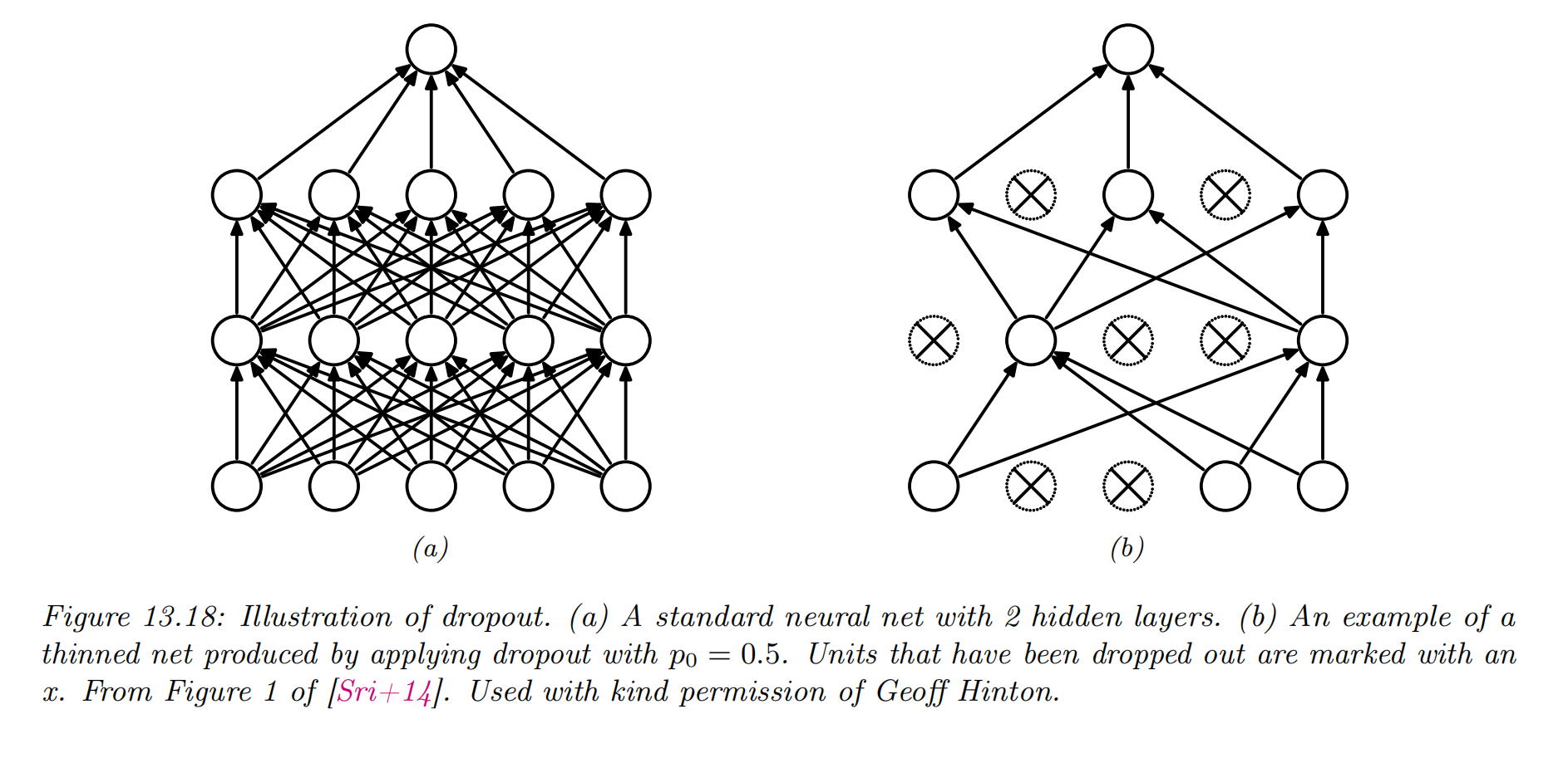
• Dropout can dramatically reduce overfitting and is very widely used.
• it prevents complex co-adaptation of the hidden units.

---

Bayesian neural networks

• Modern DNNs are usually trained using a (penalized) maximum likelihood objective to find a single setting of parameters.
• with large models, there are often many more parameters than data points
• there may be multiple possible models which fit the training data equally well, yet which generalize in different ways.
• It is often useful to capture the induced uncertainty in the posterior predictive distribution
  $$p(y \mid x, \mathcal{D})=\int p(y \mid x, \theta) p(\boldsymbol{\theta} \mid \mathcal{D}) d \boldsymbol{\theta}$$
• Bayesian neural network or BNN.
  • It can be thought of as an infinite ensemble of differently weight neural networks.
  • By marginalizing out the parameters, we can avoid overfitting.