Trees, Forests, Bagging, and Boosting

Materials are adopted from "Murphy, Kevin P. Probabilistic machine learning: an introduction. MIT press, 2022.". This handout is only for teaching. DO NOT DISTRIBUTE.

Classification and regression trees (CART)

• CART / Decision Tree
  • recursively partitioning the input space
  • a local model in each resulting region of input space

Model definition

• regression trees: all inputs are real-valued.
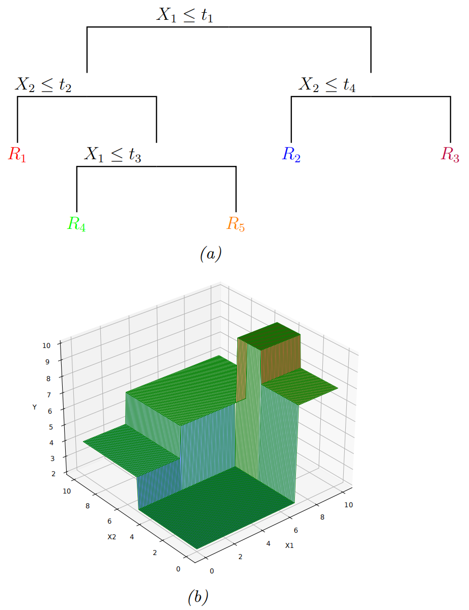
  • The tree consists of a set of nested decision rules. At each node $i$, the feature dimension $d_{i}$ of the input vector $\boldsymbol{x}$ is compared to a threshold value $t_{i}$, and the input is then passed down to the left or right branch, depending on whether it is above or below threshold.
  • At the leaves of the tree, the model specifies the predicted output for any input that falls into that part of the input space.

• An example:
  • the region of space:
    $$R_{1}=\left\{\boldsymbol{x}: x_{1} \leq t_{1}, x_{2} \leq t_{2}\right\}$$
  • the output for region 1 (mean response) can be estimated using
    $$w_{1}=\frac{\sum_{n=1}^{N} y_{n} \mathbb{I}\left(\boldsymbol{x}_{n} \in R_{1}\right)}{\sum_{n=1}^{N} \mathbb{I}\left(\boldsymbol{x}_{n} \in R_{1}\right)}$$
• Formally, a regression tree can be defined by
  $$f(\boldsymbol{x} ; \boldsymbol{\theta})=\sum_{j=1}^{J} w_{j} \mathbb{I}\left(\boldsymbol{x} \in R_{j}\right)$$
  • $R_{j}$ is the region specified by the $j$'th leaf node, $w_{j}$ is the predicted output for that node, and $\boldsymbol{\theta}=\left\{\left(R_{j}, w_{j}\right): j=1: J\right\}$
  • $J$ is the number of nodes.
  • The regions：
    • $R_{1}=\left[\left(d_{1} \leq t_{1}\right),\left(d_{2} \leq t_{2}\right)\right]$
    • $R_{2}=\left[\left(d_{1} \leq t_{1}\right),\left(d_{2}>t_{2}\right),\left(d_{3} \leq t_{3}\right)\right]$, etc.
  • For categorical inputs, we can define the splits based on comparing feature $d_{i}$ to each of the possible values for that feature, rather than comparing to a numeric threshold.

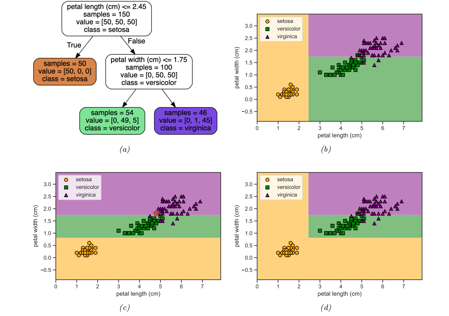
• For classification problems, the leaves contain a distribution over the class labels, rather than just the mean response.

Model fitting

• minimizing the following loss:
  $$\mathcal{L}(\boldsymbol{\theta})=\sum_{n=1}^{N} \ell\left(y_{n}, f\left(\boldsymbol{x}_{n} ; \boldsymbol{\theta}\right)\right)=\sum_{j=1}^{J} \sum_{\boldsymbol{x}_{n} \in R_{j}} \ell\left(y_{n}, w_{j}\right)$$

  • it is not differentiable
  • finding the optimal partitioning of the data is NP-complete
  • the standard practice is to use a greedy procedure, in which we iteratively grow the tree one node at a time.
  • three popular implementations: CART, C4.5, and ID3.

• the big idea of greedy algorithms

  • let $\mathcal{D}_{i}=\left\{\left(\boldsymbol{x}_{n}, y_{n}\right) \in N_{i}\right\}$ be the set of examples that reach node $i$.

  • If the $j$'the feature is a real-valued scalar

    • partition the data at node $i$ by comparing to a threshold $t$
    • the set of possible thresholds $\mathcal{T}_{j}$ for feature $j$ can be obtained by sorting the unique values of $\left\{x_{n j}\right\}$
    • example: if feature 1 has the values $\{4.5,-12,72,-12\}$, then we set $\mathcal{T}_{1}=\{-12,4.5,72\}$. For each possible threshold, we define the left and right splits, $\mathcal{D}_{i}^{L}(j, t)=\left\{\left(\boldsymbol{x}_{n}, y_{n}\right) \in N_{i}: x_{n, j} \leq t\right\}$ and $\mathcal{D}_{i}^{R}(j, t)=\left\{\left(\boldsymbol{x}_{n}, y_{n}\right) \in N_{i}: x_{n, j}>t\right\}$.

  • If the $j$'th feature is categorical with $K_{j}$ possible values

    • check if the feature is equal to each of those values or not.
    • it defines a set of $K_{j}$ possible binary splits: $\mathcal{D}_{i}^{L}(j, t)=\left\{\left(\boldsymbol{x}_{n}, y_{n}\right) \in N_{i}\right.$ : $\left.x_{n, j}=t\right\}$ and $\mathcal{D}_{i}^{R}(j, t)=\left\{\left(\boldsymbol{x}_{n}, y_{n}\right) \in N_{i}: x_{n, j} \neq t\right\}$.)

  • choose the best feature $j_{i}$ to split on, and the best value for that feature, $t_{i}$, as follows:
    $$\left(j_{i}, t_{i}\right)=\arg \min _{j \in\{1, \ldots, D\}} \min _{t \in \mathcal{T}_{j}} \frac{\left|\mathcal{D}_{i}^{L}(j, t)\right|}{\left|\mathcal{D}_{i}\right|} c\left(\mathcal{D}_{i}^{L}(j, t)\right)+\frac{\left|\mathcal{D}_{i}^{R}(j, t)\right|}{\left|\mathcal{D}_{i}\right|} c\left(\mathcal{D}_{i}^{R}(j, t)\right)$$

• the cost function $c\left(\mathcal{D}_{i}\right)$ of node $i$.

  • For regression, we can use the mean squared error
    $$\operatorname{cost}\left(\mathcal{D}_{i}\right)=\frac{1}{|\mathcal{D}|} \sum_{n \in \mathcal{D}_{i}}\left(y_{n}-\bar{y}\right)^{2}$$
    where $\bar{y}=\frac{1}{|\mathcal{D}|} \sum_{n \in \mathcal{D}_{i}} y_{n}$ is the mean of the response variable for examples reaching node $i$.
  • For classification, we first compute the empirical distribution over class labels for this node:
    $$\hat{\pi}_{i c}=\frac{1}{\left|\mathcal{D}_{i}\right|} \sum_{n \in \mathcal{D}_{i}} \mathbb{I}\left(y_{n}=c\right)$$
    Given this, we can then compute the Gini index
    $$G_{i}=\sum_{c=1}^{C} \hat{\pi}_{i c}\left(1-\hat{\pi}_{i c}\right)=\sum_{c} \hat{\pi}_{i c}-\sum_{c} \hat{\pi}_{i c}^{2}=1-\sum_{c} \hat{\pi}_{i c}^{2}$$
    This is the expected error rate. To see this, note that $\hat{\pi}_{i c}$ is the probability a random entry in the leaf belongs to class $c$, and $1-\hat{\pi}_{i c}$ is the probability it would be misclassified.

• Alternatively we can define cost as the entropy or deviance of the node:
  $$H_{i}=\mathbb{H}\left(\hat{\boldsymbol{\pi}}_{i}\right)=-\sum_{c=1}^{C} \hat{\pi}_{i c} \log \hat{\pi}_{i c}$$

  • A node that is pure (i.e., only has examples of one class) will have 0 entropy.

Regularization

• the danger of overfitting: If we let the tree become deep enough, it can achieve 0 error on the training set (assuming no label noise), by partioning the input space into sufficiently small regions where the output is constant.
• two main approaches against overfitting:
  • The first is to stop the tree growing process according to some heuristic, such as having too few examples at a node, or reaching a maximum depth.
  • The second approach is to grow the tree to its maximum depth, where no more splits are possible, and then to prune it back, by merging split subtrees back into their parent.

Pros and cons

• advantages:

  • They are easy to interpret.
  • They can easily handle mixed discrete and continuous inputs.
  • They are insensitive to monotone transformations of the inputs (because the split points are based on ranking the data points), so there is no need to standardize the data.
  • They perform automatic variable selection.
  • They are relatively robust to outliers.
  • They are fast to fit, and scale well to large data sets.
  • They can handle missing input features.

• disadvantages:

  • they do not predict very accurately compared to other kinds of model (the greedy nature of the tree construction algorithm).
  • trees are unstable: small changes to the input data can have large effects on the structure of the tree, due to the hierarchical nature of the tree-growing process, causing errors at the top to affect the rest of the tree.

Ensemble learning

• Ensemble learning: reduce variance by averaging multiple (regression) models (or taking a majority vote for classifiers)
  $$f(y \mid \boldsymbol{x})=\frac{1}{|\mathcal{M}|} \sum_{m \in \mathcal{M}} f_{m}(y \mid \boldsymbol{x})$$

  • $f_{m}$ is the $m$'th base model.
  • The ensemble will have similar bias to the base models, but lower variance, generally resulting in improved overall performance

• For classifiers: take a majority vote of the outputs. (This is sometimes called a committee method.)

  • suppose each base model is a binary classifier with an accuracy of $\theta$, and suppose class 1 is the correct class.
  • Let $Y_{m} \in\{0,1\}$ be the prediction for the $m$'th model
  • Let $S=\sum_{m=1}^{M} Y_{m}$ be the number of votes for class 1
  • We define the final predictor to be the majority vote, i.e., class 1 if $S>M / 2$ and class 0 otherwise. The probability that the ensemble will pick class 1 is
    $$p=\operatorname{Pr}(S>M / 2)=1-B(M / 2, M, \theta)$$

Stecking

• Stecking (stacked generalization): combine the base models, by using
  $$f(y \mid \boldsymbol{x})=\sum_{m \in \mathcal{M}} w_{m} f_{m}(y \mid \boldsymbol{x})$$
  • the combination weights used by stacking need to be trained on a separate dataset, otherwise they would put all their mass on the best performing base model.

Ensembling is not Bayes model averaging

• An ensemble considers a larger hypothesis class of the form
  $$p(y \mid \boldsymbol{x}, \boldsymbol{w}, \boldsymbol{\theta})=\sum_{m \in \mathcal{M}} w_{m} p\left(y \mid \boldsymbol{x}, \boldsymbol{\theta}_{m}\right)$$

• the BMA uses
  $$p(y \mid \boldsymbol{x}, \mathcal{D})=\sum_{m \in \mathcal{M}} p(m \mid \mathcal{D}) p(y \mid \boldsymbol{x}, m, \mathcal{D})$$

• The key difference

  • in the case of BMA, the weights $p(m \mid \mathcal{D})$ sum to one
  • in the limit of infinite data, only a single model will be chosen (namely the MAP model). By contrast,
  • the ensemble weights $w_{m}$ are arbitrary, and don't collapse in this way to a single model.

Bagging

• bagging ("bootstrap aggregating")

  • This is a simple form of ensemble learning in which we fit $M$ different base models to different randomly sampled versions of the data
  • this encourages the different models to make diverse predictions
  • The datasets are sampled with replacement (a technique known as bootstrap sampling)
  • a given example may appear multiple times, until we have a total of $N$ examples per model (where $N$ is the number of original data points).

• The disadvantage of bootstrap

  • each base model only sees, on average, $63 \%$ of the unique input examples.

  • The $37 \%$ of the training instances that are not used by a given base model are called out-of-bag instances (oob).

  • We can use the predicted performance of the base model on these oob instances as an estimate of test set performance.

  • This provides a useful alternative to cross validation.

• The main advantage of bootstrap is that it prevents the ensemble from relying too much on any individual training example, which enhances robustness and generalization.

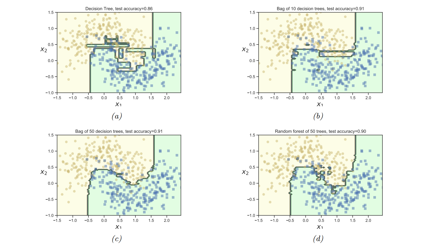
• Bagging does not always improve performance. In particular, it relies on the base models being unstable estimators (decision tree), so that omitting some of the data significantly changes the resulting model fit.

Random forests

Random forests: learning trees based on a randomly chosen subset of input variables (at each node of the tree), as well as a randomly chosen subset of data cases.

Figure 18.5 shows that random forests work much better than bagged decision trees, because many input features are irrelevant.

Boosting

• Ensembles of trees, whether fit by bagging or the random forest algorithm, corresponding to a model of the form
  $$f(\boldsymbol{x} ; \boldsymbol{\theta})=\sum_{m=1}^{M} \beta_{m} F_{m}\left(\boldsymbol{x} ; \boldsymbol{\theta}_{m}\right)$$

  • $F_{m}$ is the $m$'th tree
  • $\beta_{m}$ is the corresponding weight, often set to $\beta_{m}=1$.

• additive model: generalize this by allowing the $F_{m}$ functions to be general function approximators, such as neural networks, not just trees.

• We can think of this as a linear model with adaptive basis functions. The goal, as usual, is to minimize the empirical loss (with an optional regularizer):
  $$\mathcal{L}(f)=\sum_{i=1}^{N} \ell\left(y_{i}, f\left(\boldsymbol{x}_{i}\right)\right)$$

• Boosting is an algorithm for sequentially fitting additive models where each $F_{m}$ is a binary classifier that returns $F_{m} \in\{-1,+1\}$.

  • first fit $F_{1}$ on the original data
  • weight the data samples by the errors made by $F_{1}$, so misclassified examples get more weight
  • fit $F_{2}$ to this weighted data set
  • keep repeating this process until we have fit the desired number $M$ of components.

• as long as each $F_{m}$ has an accuracy that is better than chance (even on the weighted dataset), then the final ensemble of classifiers will have higher accuracy than any given component.

  • if $F_{m}$ is a weak learner (so its accuracy is only slightly better than $50 \%$ )
  • we can boost its performance using the above procedure so that the final $f$ becomes a strong learner.

• boosting, bagging and RF

  • boosting reduces the bias of the strong learner, by fitting trees that depend on each other
  • bagging and RF reduce the variance by fitting independent trees
  • In many cases, boosting can work better

Forward stagewise additive modeling

forward stagewise additive modeling: sequentially optimize the objective for general (differentiable) loss functions
$$\left(\beta_{m}, \boldsymbol{\theta}_{m}\right)=\underset{\beta, \boldsymbol{\theta}}{\operatorname{argmin}} \sum_{i=1}^{N} \ell\left(y_{i}, f_{m-1}\left(\boldsymbol{x}_{i}\right)+\beta F\left(\boldsymbol{x}_{i} ; \boldsymbol{\theta}\right)\right)$$
We then set
$$f_{m}(\boldsymbol{x})=f_{m-1}(\boldsymbol{x})+\beta_{m} F\left(\boldsymbol{x} ; \boldsymbol{\theta}_{m}\right)=f_{m-1}(\boldsymbol{x})+\beta_{m} F_{m}(\boldsymbol{x})$$

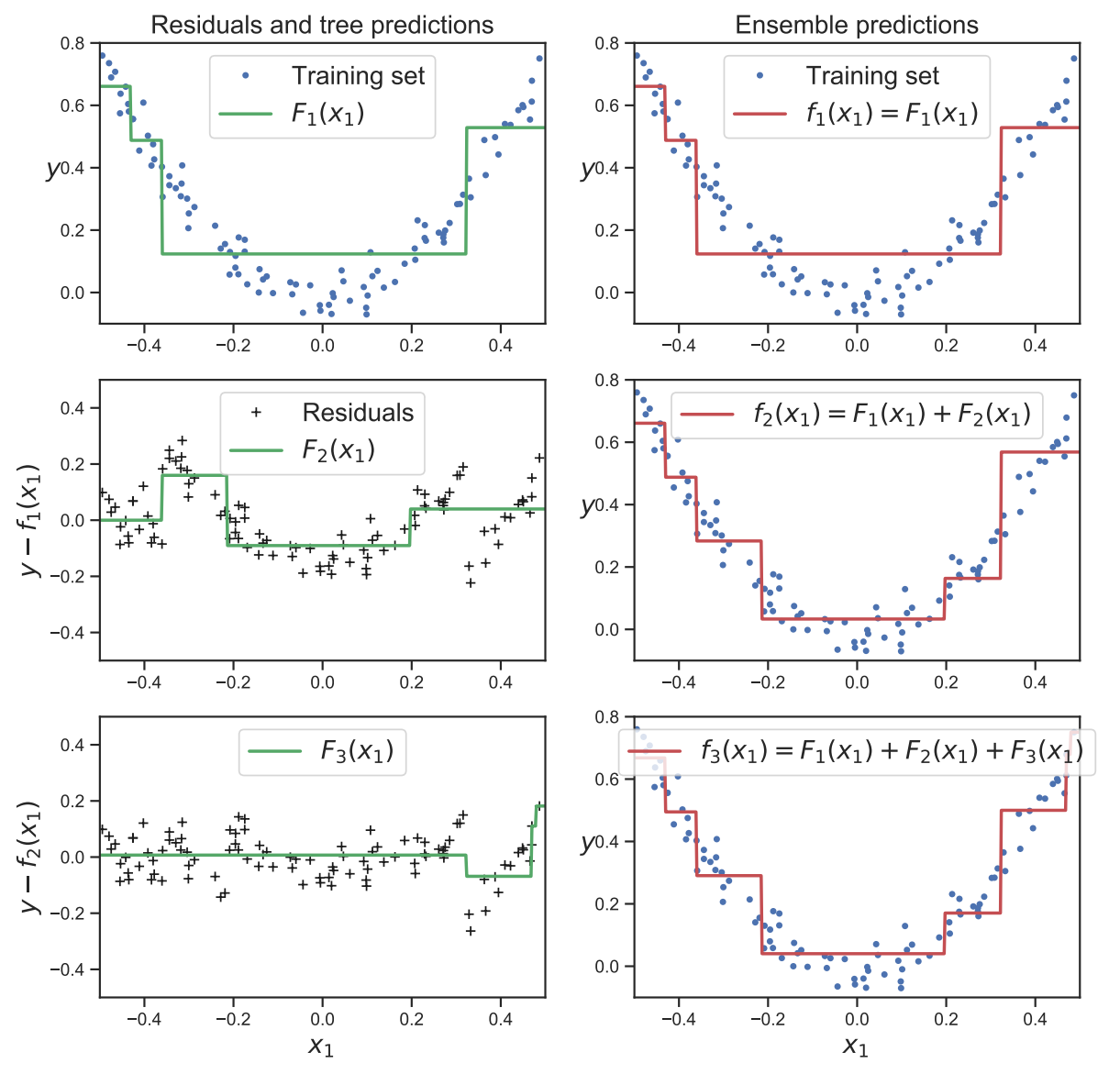
Quadratic loss and least squares boosting

• squared error loss $\ell(y, \hat{y})=(y-\hat{y})^{2}$
• the $i$'th term in the objective at step $m$ becomes
  $$\ell\left(y_{i}, f_{m-1}\left(\boldsymbol{x}_{i}\right)+\beta F\left(\boldsymbol{x}_{i} ; \boldsymbol{\theta}\right)\right)=\left(y_{i}-f_{m-1}\left(\boldsymbol{x}_{i}\right)-\beta F\left(\boldsymbol{x}_{i} ; \boldsymbol{\theta}\right)\right)^{2}=\left(r_{i m}-\beta F\left(\boldsymbol{x}_{i} ; \boldsymbol{\theta}\right)\right)^{2}$$
  • $r_{i m}=y_{i}-f_{m-1}\left(\boldsymbol{x}_{i}\right)$ is the residual of the current model on the $i$'th observation.
• We can minimize the above objective by simply setting $\beta=1$, and fitting $F$ to the residual errors. This is called least squares boosting.

Exponential loss and AdaBoost

• binary classification, i.e., predicting $\tilde{y}_{i} \in\{-1,+1\}$.

• assuming the weak learner computes
  $$p(y=1 \mid \boldsymbol{x})=\frac{e^{F(\boldsymbol{x})}}{e^{-F(\boldsymbol{x})}+e^{F(\boldsymbol{x})}}=\frac{1}{1+e^{-2 F(\boldsymbol{x})}}$$
  so $F(\boldsymbol{x})$ returns half the log odds.

• the negative log likelihood is given by
  $$\ell(\tilde{y}, F(\boldsymbol{x}))=\log \left(1+e^{-2 \tilde{y} F(\boldsymbol{x})}\right)$$

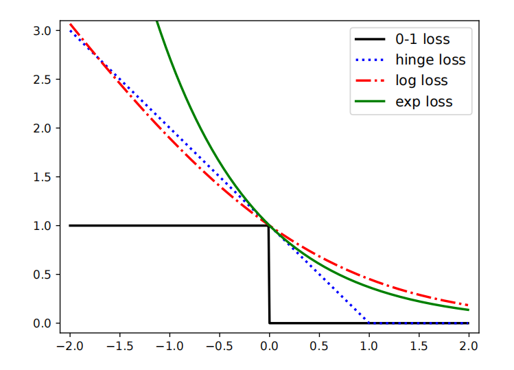
• we can also use other loss functions. In this section, we consider the exponential loss
  $$\ell(\tilde{y}, F(\boldsymbol{x}))=\exp (-\tilde{y} F(\boldsymbol{x}))$$

• this is a smooth upper bound on the 0-1 loss.
• In the population setting (with infinite sample size), the optimal solution to the exponential loss is the same as for $\log$ loss. To see this, we can just set the derivative of the expected loss (for each $\boldsymbol{x}$ ) to zero:
  $$\begin{aligned} \frac{\partial}{\partial F(\boldsymbol{x})} \mathbb{E}\left[e^{-\tilde{y} f(\boldsymbol{x})} \mid x\right] &=\frac{\partial}{\partial F(\boldsymbol{x})}\left[p(\tilde{y}=1 \mid \boldsymbol{x}) e^{-F(\boldsymbol{x})}+p(\tilde{y}=-1 \mid x) e^{F(\boldsymbol{x})}\right] \\ &=-p(\tilde{y}=1 \mid \boldsymbol{x}) e^{-F(\boldsymbol{x})}+p(\tilde{y}=-1 \mid x) e^{F(\boldsymbol{x})} \\ &=0 \Rightarrow \frac{p(\tilde{y}=1 \mid \boldsymbol{x})}{p(\tilde{y}=-1 \mid \boldsymbol{x})}=e^{2 F(\boldsymbol{x})} \end{aligned}$$
• the exponential loss is easier to optimize in the boosting setting.

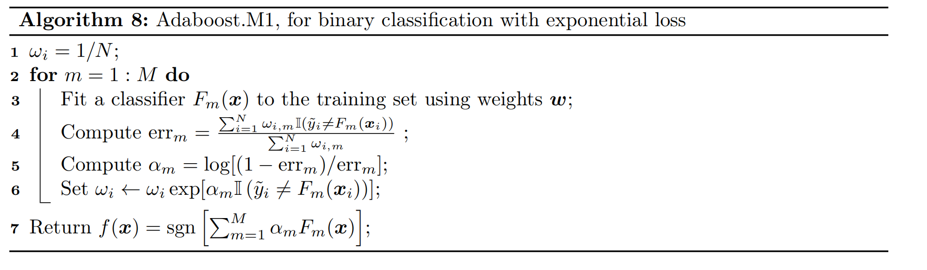
discrete AdaBoost

• At step $m$ we have to minimize
  $$L_{m}(F)=\sum_{i=1}^{N} \exp \left[-\tilde{y}_{i}\left(f_{m-1}\left(\boldsymbol{x}_{i}\right)+\beta F\left(\boldsymbol{x}_{i}\right)\right)\right]=\sum_{i=1}^{N} \omega_{i, m} \exp \left(-\beta \tilde{y}_{i} F\left(\boldsymbol{x}_{i}\right)\right)$$

where $\omega_{i, m} \triangleq \exp \left(-\tilde{y}_{i} f_{m-1}\left(\boldsymbol{x}_{i}\right)\right)$ is a weight applied to datacase $i$, and $\tilde{y}_{i} \in\{-1,+1\}$. We can rewrite this objective as follows:
$$\begin{aligned} L_{m} &=e^{-\beta} \sum_{\tilde{y}_{i}=F\left(\boldsymbol{x}_{i}\right)} \omega_{i, m}+e^{\beta} \sum_{\tilde{y}_{i} \neq F\left(\boldsymbol{x}_{i}\right)} \omega_{i, m} \\ &=\left(e^{\beta}-e^{-\beta}\right) \sum_{i=1}^{N} \omega_{i, m} \mathbb{I}\left(\tilde{y}_{i} \neq F\left(\boldsymbol{x}_{i}\right)\right)+e^{-\beta} \sum_{i=1}^{N} \omega_{i, m} \end{aligned}$$

• the optimal function to add is
  $$F_{m}=\underset{F}{\operatorname{argmin}} \sum_{i=1}^{N} \omega_{i, m} \mathbb{I}\left(\tilde{y}_{i} \neq F\left(\boldsymbol{x}_{i}\right)\right)$$
  This can be found by applying the weak learner to a weighted version of the dataset, with weights $\omega_{i, m}$.

• Subsituting $F_{m}$ into $L_{m}$ and solving for $\beta$ we find
  $$\beta_{m}=\frac{1}{2} \log \frac{1-\operatorname{err}_{m}}{\operatorname{err}_{m}}$$
  where
  $$\operatorname{err}_{m}=\frac{\sum_{i=1}^{N} \omega_{i, m} \mathbb{I}\left(\tilde{y}_{i} \neq F_{m}\left(\boldsymbol{x}_{i}\right)\right)}{\sum_{i=1}^{N} \omega_{i, m}}$$

• Therefore overall update becomes
  $$f_{m}(\boldsymbol{x})=f_{m-1}(\boldsymbol{x})+\beta_{m} F_{m}(\boldsymbol{x})$$

• the weights for the next iteration, as follows:
  $$\omega_{i, m+1}=e^{-\tilde{y}_{i} f_{m}\left(\boldsymbol{x}_{i}\right)}=e^{-\tilde{y}_{i} f_{m-1}\left(\boldsymbol{x}_{i}\right)-\tilde{y}_{i} \beta_{m} F_{m}\left(\boldsymbol{x}_{i}\right)}=\omega_{i, m} e^{-\tilde{y}_{i} \beta_{m} F_{m}\left(\boldsymbol{x}_{i}\right)}$$

• If $\tilde{y}_{i}=F_{m}\left(\boldsymbol{x}_{i}\right)$, then $\tilde{y}_{i} F_{m}\left(\boldsymbol{x}_{i}\right)=1$, and if $\tilde{y}_{i} \neq F_{m}\left(\boldsymbol{x}_{i}\right)$, then $\tilde{y}_{i} F_{m}\left(\boldsymbol{x}_{i}\right)=-1$. Hence $-\tilde{y}_{i} F_{m}\left(\boldsymbol{x}_{i}\right)=$ $2 \mathbb{I}\left(\tilde{y}_{i} \neq F_{m}\left(\boldsymbol{x}_{o}\right)\right)-1$, so the update becomes
  $$\omega_{i, m+1}=\omega_{i, m} e^{\beta_{m}\left(2 \mathbb{I}\left(\tilde{y}_{i} \neq F_{m}\left(\boldsymbol{x}_{i}\right)\right)-1\right)}=\omega_{i, m} e^{2 \beta_{m} \mathbb{I}\left(\tilde{y}_{i} \neq F_{m}\left(\boldsymbol{x}_{i}\right)\right)} e^{-\beta_{m}}$$

• Since the $e^{-\beta_{m}}$ is constant across all examples, it can be dropped. If we then define $\alpha_{m}=2 \beta_{m}$, the update becomes
  $$\omega_{i, m+1}= \begin{cases}\omega_{i, m} e^{\alpha_{m}} & \text { if } \tilde{y}_{i} \neq F_{m}\left(\boldsymbol{x}_{i}\right) \\ \omega_{i, m} & \text { otherwise }\end{cases}$$
  Thus we see that we exponentially increase weights of misclassified examples. The resulting algorithm shown in Algorithm 8, and is known as Adaboost.M1 [FS96].

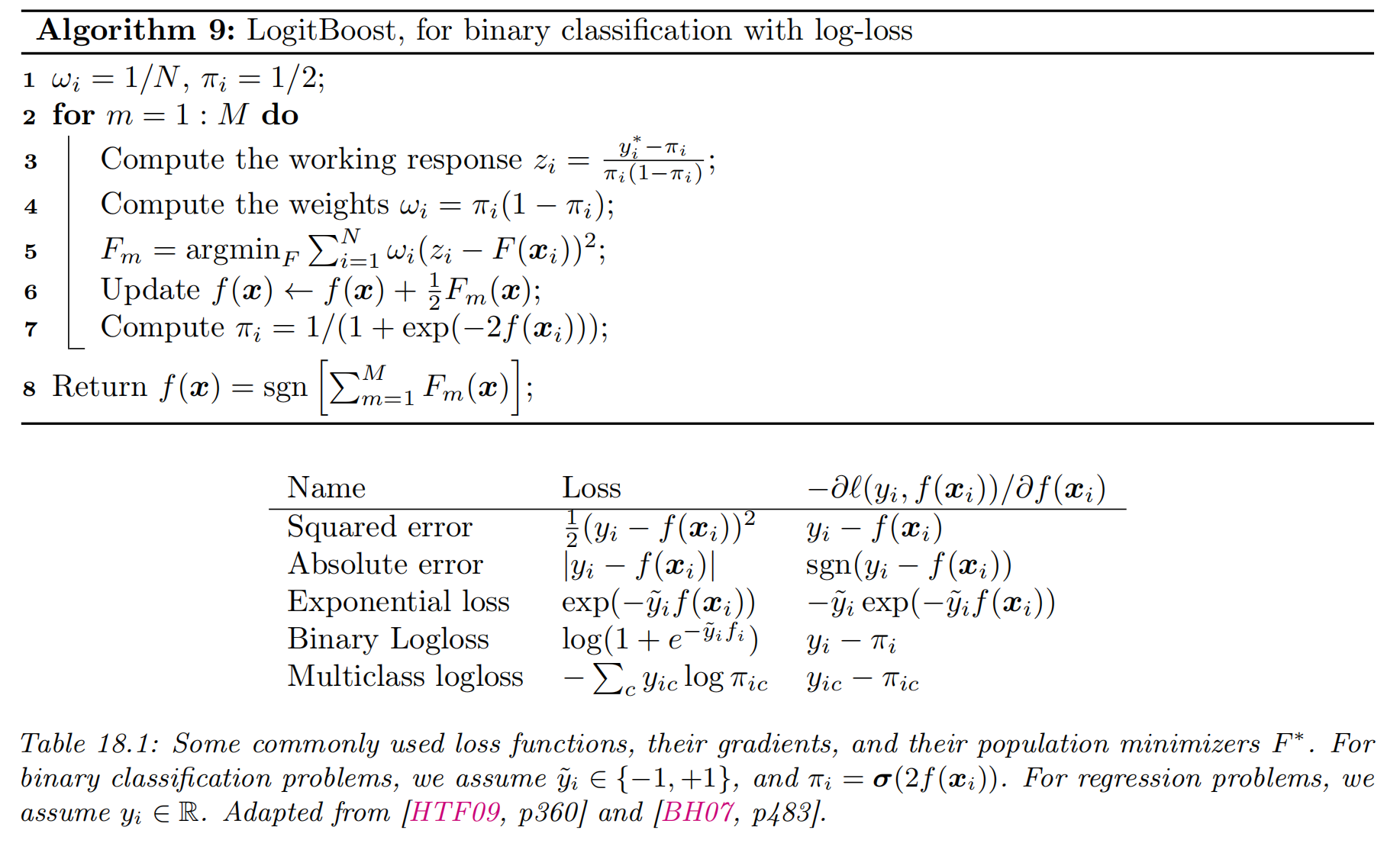
LogitBoost

• exponential loss puts a lot of weight on misclassified examples
• This makes the method very sensitive to outliers (mislabeled examples).
• In addition, $e^{-\tilde{y} f}$ is not the logarithm of any pmf for binary variables $\tilde{y} \in\{-1,+1\}$; consequently we cannot recover probability estimates from $f(\boldsymbol{x})$.
• A natural alternative is to use $\log$ loss. This only punishes mistakes linearly, as is clear from Figure 18.7.
• Furthermore, it means that we will be able to extract probabilities from the final learned function, using
  $$p(y=1 \mid x)=\frac{e^{f(\boldsymbol{x})}}{e^{-f(\boldsymbol{x})}+e^{f(\boldsymbol{x})}}=\frac{1}{1+e^{-2 f(\boldsymbol{x})}}$$
• The goal is to minimze the expected log-loss, given by
  $$L_{m}(F)=\sum_{i=1}^{N} \log \left[1+\exp \left(-2 \tilde{y}_{i}\left(f_{m-1}(\boldsymbol{x})+F\left(\boldsymbol{x}_{i}\right)\right)\right)\right]$$

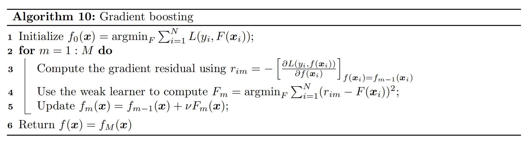
Gradient boosting

• to derive a generic version, known as gradient boosting. To explain this, imagine solving $\hat{\boldsymbol{f}}=\operatorname{argmin}_{\boldsymbol{f}} \mathcal{L}(\boldsymbol{f})$ by performing gradient descent in the space of functions. Since functions are infinite dimensional objects, we will represent them by their values on the training set, $\boldsymbol{f}=\left(f\left(\boldsymbol{x}_{1}\right), \ldots, f\left(\boldsymbol{x}_{N}\right)\right)$. At step $m$, let $\boldsymbol{g}_{m}$ be the gradient of $\mathcal{L}(\boldsymbol{f})$ evaluated at $\boldsymbol{f}=\boldsymbol{f}_{m-1}$ :
  $$g_{i m}=\left[\frac{\partial \ell\left(y_{i}, f\left(\boldsymbol{x}_{i}\right)\right)}{\partial f\left(\boldsymbol{x}_{i}\right)}\right]_{f=f_{m-1}}$$

• make the update
  $$\boldsymbol{f}_{m}=\boldsymbol{f}_{m-1}-\beta_{m} \boldsymbol{g}_{m}$$
  where $\beta_{m}$ is the step length, chosen by
  $$\beta_{m}=\underset{\beta}{\operatorname{argmin}} \mathcal{L}\left(\boldsymbol{f}_{m-1}-\beta \boldsymbol{g}_{m}\right)$$
• fitting a weak learner to approximate the negative gradient signal. That is, we use this update
  $$F_{m}=\underset{F}{\operatorname{argmin}} \sum_{i=1}^{N}\left(-g_{i m}-F\left(\boldsymbol{x}_{i}\right)\right)^{2}$$

If we apply this algorithm using squared loss, we recover L2Boosting, since $-g_{i m}=y_{i}-f_{m-1}\left(\boldsymbol{x}_{i}\right)$ is just the residual error. We can also apply this algorithm to other loss functions, such as absolute loss or Huber loss (Section 5.1.5.3), which is useful for robust regression problems.

For classification, we can use log-loss. In this case, we get an algorithm known as BinomialBoost [BH07]. The advantage of this over LogitBoost is that it does not need to be able to do weighted fitting: it just applies any black-box regression model to the gradient vector. To apply this to multi-class classification, we can fit $C$ separate regression trees, using the pseudo residual of the form
$$-g_{i c m}=\frac{\partial \ell\left(y_{i}, f_{1 m}\left(\boldsymbol{x}_{i}\right), \ldots, f_{C m}\left(\boldsymbol{x}_{i}\right)\right)}{\partial f_{c m}\left(\boldsymbol{x}_{i}\right)}=\mathbb{I}\left(y_{i}=c\right)-\pi_{i c}$$
Although the trees are fit separately, their predictions are combined via a softmax transform
$$p(y=c \mid \boldsymbol{x})=\frac{e^{f_{c}(\boldsymbol{x})}}{\sum_{c^{\prime}=1}^{C} e^{f_{c^{\prime}}(\boldsymbol{x})}}$$
When we have large datasets, we can use a stochastic variant in which we subsample (without replacement) a random fraction of the data to pass to the regression tree at each iteration. This is called stochastic gradient boosting [Fri99]. Not only is it faster, but it can also generalize better, because subsampling the data is a form of regularization.

Gradient tree boosting

In practice, gradient boosting nearly always assumes that the weak learner is a regression tree, which is a model of the form
$$F_{m}(\boldsymbol{x})=\sum_{j=1}^{J_{m}} w_{j m} \mathbb{I}\left(\boldsymbol{x} \in R_{j m}\right)$$
where $w_{j m}$ is the predicted output for region $R_{j m}$. (In general, $w_{j m}$ could be a vector.) This combination is called gradient boosted regression trees, or gradient tree boosting. (A related version is known as MART, which stands for "multivariate additive regression trees" [FM03].)
To use this in gradient boosting, we first find good regions $R_{j m}$ for tree $m$ using standard regression tree learning (see Section 18.1) on the residuals; we then (re)solve for the weights of each leaf by solving
$$\hat{w}_{j m}=\underset{w}{\operatorname{argmin}} \sum_{\boldsymbol{x}_{i} \in R_{j m}} \ell\left(y_{i}, f_{m-1}\left(\boldsymbol{x}_{i}\right)+w\right)$$

XGBoost

• XGBoost: (https://github.com/dmlc/xgboost), which stands for "extreme gradient boosting".is a very efficient and widely used implementation of gradient boosted trees:
  • it adds a regularizer on the tree complexity
  • it uses a second order approximation of the loss instead of just a linear approximation
  • it samples features at internal nodes (as in random forests)
  • it uses various computer science methods (such as handling out-of-core computation for large datasets) to ensure scalability.
• In more detail, XGBoost optimizes the following regularized objective
  $$\mathcal{L}(f)=\sum_{i=1}^{N} \ell\left(y_{i}, f\left(\boldsymbol{x}_{i}\right)\right)+\Omega(f)$$
• the regularizer
  $$\Omega(f)=\gamma J+\frac{1}{2} \lambda \sum_{j=1}^{J} w_{j}^{2}$$
  where $J$ is the number of leaves, and $\gamma \geq 0$ and $\lambda \geq 0$ are regularization coefficients.
• At the $m$'th step, the loss is given by
  $$\mathcal{L}_{m}\left(F_{m}\right)=\sum_{i=1}^{N} \ell\left(y_{i}, f_{m-1}\left(\boldsymbol{x}_{i}\right)+F_{m}\left(\boldsymbol{x}_{i}\right)\right)+\Omega\left(F_{m}\right)+\text { const }$$
• the second order Taylor expansion:
  $$\mathcal{L}_{m}\left(F_{m}\right) \approx \sum_{i=1}^{N}\left[\ell\left(y_{i}, f_{m-1}\left(\boldsymbol{x}_{i}\right)\right)+g_{i m} F_{m}\left(\boldsymbol{x}_{i}\right)+\frac{1}{2} h_{i m} F_{m}^{2}\left(\boldsymbol{x}_{i}\right)\right]+\Omega\left(F_{m}\right)+\text { const }$$
  where $h_{i m}$ is the Hessian
  $$h_{i m}=\left[\frac{\partial^{2} \ell\left(y_{i}, f\left(\boldsymbol{x}_{i}\right)\right)}{\partial f\left(\boldsymbol{x}_{i}\right)^{2}}\right]_{f=f_{m-1}}$$
  In the case of regression trees, we have $F(\boldsymbol{x})=w_{q(\boldsymbol{x})}$, where $q: \mathbb{R}^{D} \rightarrow\{1, \ldots, J\}$ specifies which leaf node $\boldsymbol{x}$ belongs to, and $\boldsymbol{w} \in \mathbb{R}^{J}$ are the leaf weights. Hence we can rewrite Equation (18.49) as

follows, dropping terms that are independent of $F_{m}$ :
$$\begin{aligned} \mathcal{L}_{m}(q, \boldsymbol{w}) & \approx \sum_{i=1}^{N}\left[g_{i m} F_{m}\left(\boldsymbol{x}_{i}\right)+\frac{1}{2} h_{i m} F_{m}^{2}\left(\boldsymbol{x}_{i}\right)\right]+\gamma J+\frac{1}{2} \lambda \sum_{j=1}^{J} w_{j}^{2} \\ &=\sum_{j=1}^{J}\left[\left(\sum_{i \in I_{j}} g_{i m}\right) w_{j}+\frac{1}{2}\left(\sum_{i \in I_{j}} h_{i}+\lambda\right) w_{j}^{2}\right]+\gamma J \end{aligned}$$
where $I_{j}=\left\{i: q\left(\boldsymbol{x}_{i}\right)=j\right\}$ is the set of indices of data points assigned to the $j$ 'th leaf.
Let us define $G_{j m}=\sum_{i \in I_{j}} g_{i m}$ and $H_{j m}=\sum_{i \in I_{j}} h_{i m}$. Then the above simplifies to
$$\mathcal{L}_{m}(q, \boldsymbol{w})=\sum_{j=1}^{J}\left[G_{j m} w_{j}+\frac{1}{2}\left(H_{j m}+\lambda\right) w_{j}^{2}\right]+\gamma J$$
This is a quadratic in each $w_{j} \mathrm{~m}$ so the optimal weights are given by
$$w_{j}^{*}=-\frac{G_{j m}}{H_{j m}+\lambda}$$
The loss for evaluating different tree structures $q$ then becomes
$$\mathcal{L}_{m}\left(q, \boldsymbol{w}^{*}\right)=-\frac{1}{2} \sum_{j=1}^{J} \frac{G_{j m}^{2}}{H_{j m}+\lambda}+\gamma J$$
We can greedily optimize this using a recursive node splitting procedure, as in Section 18.1. Specifically, for a given leaf $j$, we consider splitting it into a left and right half, $I=I_{L} \cup I_{R}$. We can compute the gain (reduction in loss) of such a split as follows:
$$\text { gain }=\frac{1}{2}\left[\frac{G_{L}^{2}}{H_{L}+\lambda}+\frac{G_{R}^{2}}{H_{R}+\lambda}-\frac{\left(G_{L}+G_{R}\right)^{2}}{\left(H_{L}+H_{R}\right)+\lambda}\right]-\gamma$$
where $G_{L}=\sum_{i \in I_{L}} g_{i m}, G_{R}=\sum_{i \in I_{R}} g_{i m}, H_{L}=\sum_{i \in I_{L}} h_{i m}$, and $H_{R}=\sum_{i \in I_{R}} h_{i m}$. Thus we see that it is not worth splitting a node if the gain is negative (i.e., the first term is less than $\gamma$ ).

Interpreting tree ensembles

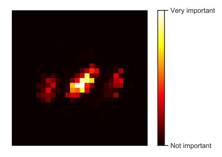
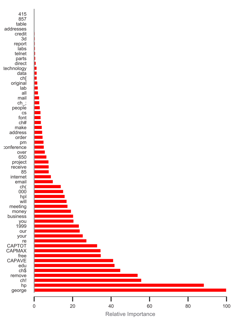
Feature importance

• For a single decision tree $T,[\mathrm{BFO} 84]$ proposed the following measure for feature importance of feature $k$ :
  $$R_{k}(T)=\sum_{j=1}^{J-1} G_{j} \mathbb{I}\left(v_{j}=k\right)$$

  • the sum is over all non-leaf (internal) nodes
  • $G_{j}$ is the gain in accuracy (reduction in cost) at node $j$
  • and $v_{j}=k$ if node $j$ uses feature $k$.

• averaging over all trees in the ensemble:
  $$R_{k}=\frac{1}{M} \sum_{m=1}^{M} R_{k}\left(T_{m}\right)$$

• normalize scores so the largest value is $100 \%$

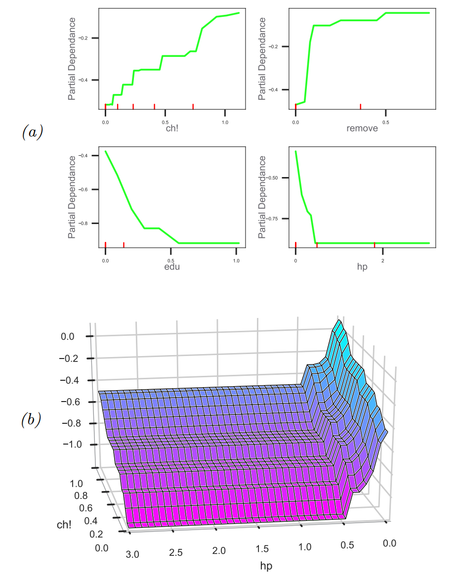
Partial dependency plots

• a partial dependency plot for feature $k$ is a plot of the following function vs $x_{k}$.
  $$\bar{f}_{k}\left(x_{k}\right)=\frac{1}{N} \sum_{n=1}^{N} f\left(\boldsymbol{x}_{n,-k}, x_{k}\right)$$

• we marginalize out all features except $k$. In the case of a binary classifier, we can convert this to $\log$ odds, $\log p\left(y=1 \mid x_{k}\right) / p\left(y=0 \mid x_{k}\right)$, before plotting.

• interaction effects between features $j$ and $k$:
  $$\bar{f}_{j k}\left(x_{j}, x_{k}\right)=\frac{1}{N} \sum_{n=1}^{N} f\left(\boldsymbol{x}_{n,-j k}, x_{j}, x_{k}\right)$$