L03 Dimensionality Reduction

Materials are adopted from "Murphy, Kevin P. Probabilistic machine learning: an introduction. MIT press, 2022.". This handout is only for teaching. DO NOT DISTRIBUTE.

Principal components analysis (PCA)

Examples

• a simple example project from 2d to 1d
  

• hand writing digit recognition (28*28d to 2d)
  

• human face recognition (64*64d to 3d)
  

Derivation of the algorithm

• (unlabeled) dataset $\mathcal{D}=\left\{\boldsymbol{x}_{n}\in \mathbb{R}^{D}: n=1: N\right\}$, where $\boldsymbol{x}_{n} \in \mathbb{R}^{D}$.

  • We can represent this as an $N \times D$ data matrix $\mathbf{X}$.
  • $\overline{\boldsymbol{x}}=\frac{1}{N} \sum_{n=1}^{N} \boldsymbol{x}_{n}=\mathbf{0}$

• approximate each $\boldsymbol{x}_{n}$ by a low dimensional representation, $\boldsymbol{z}_{n} \in \mathbb{R}^{L}$

  • linear subspace spaned by basis:$\boldsymbol{w}_{1}, \ldots, \boldsymbol{w}_{L}$, where each $\boldsymbol{w}_{k} \in \mathbb{R}^{D}$
  • encoder: $\boldsymbol{z}=\mathbf{W}^{\top}\boldsymbol{x}$
  • decoder: $\hat{\boldsymbol{x}}=\mathbf{W}\boldsymbol{z}$
  • the reconstruction error:

$$\mathcal{L}(\mathbf{W}, \mathbf{Z})=\frac{1}{N}\left\|\mathbf{X}-\mathbf{Z} \mathbf{W}^{\top}\right\|_{F}^{2}=\frac{1}{N}\left\|\mathbf{X}^{\top}-\mathbf{W} \mathbf{Z}^{\top}\right\|_{F}^{2}=\frac{1}{N} \sum_{n=1}^{N}\left\|\boldsymbol{x}_{n}-\mathbf{W} \boldsymbol{z}_{n}\right\|^{2}$$

Base case

consider the 1 dimention case: $\boldsymbol{w}_{1} \in \mathbb{R}^{D}$

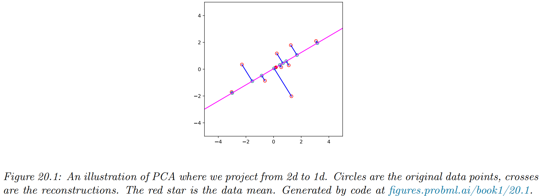
Let the coefficients for each of the data points associated with the first basis vector be denoted by $\tilde{\mathbf{z}}_{1}=\left[z_{11}, \ldots, z_{N 1}\right] \in \mathbb{R}^{N}$. The reconstruction error is given by
$$\begin{aligned} \mathcal{L}\left(\boldsymbol{w}_{1}, \tilde{\mathbf{z}}_{1}\right) &=\frac{1}{N} \sum_{n=1}^{N}\left\|\boldsymbol{x}_{n}-z_{n 1} \boldsymbol{w}_{1}\right\|^{2}=\frac{1}{N} \sum_{n=1}^{N}\left(\boldsymbol{x}_{n}-z_{n 1} \boldsymbol{w}_{1}\right)^{\top}\left(\boldsymbol{x}_{n}-z_{n 1} \boldsymbol{w}_{1}\right).\\ &=\frac{1}{N} \sum_{n=1}^{N}\left[\boldsymbol{x}_{n}^{\top} \boldsymbol{x}_{n}-2 z_{n 1} \boldsymbol{w}_{1}^{\top} \boldsymbol{x}_{n}+z_{n 1}^{2} \boldsymbol{w}_{1}^{\top} \boldsymbol{w}_{1}\right] \\ &=\frac{1}{N} \sum_{n=1}^{N}\left[\boldsymbol{x}_{n}^{\top} \boldsymbol{x}_{n}-2 z_{n 1} \boldsymbol{w}_{1}^{\top} \boldsymbol{x}_{n}+z_{n 1}^{2}\right] \end{aligned}$$

Taking derivatives wrt $z_{n 1}$ and equating to zero gives

$$\frac{\partial}{\partial z_{n 1}} \mathcal{L}\left(\boldsymbol{w}_{1}, \tilde{\mathbf{z}}_{1}\right)=\frac{1}{N}\left[-2 \boldsymbol{w}_{1}^{\top} \boldsymbol{x}_{n}+2 z_{n 1}\right]=0 \Rightarrow z_{n 1}=\boldsymbol{w}_{1}^{\top} \boldsymbol{x}_{n}$$

Plugging this back in gives the loss for the weights:

$$\mathcal{L}\left(\boldsymbol{w}_{1}\right)=\mathcal{L}\left(\boldsymbol{w}_{1}, \tilde{\mathbf{z}}_{1}^{*}\left(\boldsymbol{w}_{1}\right)\right)=\frac{1}{N} \sum_{n=1}^{N}\left[\boldsymbol{x}_{n}^{\top} \boldsymbol{x}_{n}-z_{n 1}^{2}\right]=\mathrm{const}-\frac{1}{N} \sum_{n=1}^{N} z_{n 1}^{2}$$
To solve for $\boldsymbol{w}_{1}$, note that
$$\mathcal{L}\left(\boldsymbol{w}_{1}\right)=-\frac{1}{N} \sum_{n=1}^{N} z_{n 1}^{2}=-\frac{1}{N} \sum_{n=1}^{N} \boldsymbol{w}_{1}^{\top} \boldsymbol{x}_{n} \boldsymbol{x}_{n}^{\top} \boldsymbol{w}_{1}=-\boldsymbol{w}_{1}^{\top} \hat{\boldsymbol{\Sigma}} \boldsymbol{w}_{1}$$
where $\boldsymbol{\Sigma}$ is the empirical covariance matrix (since we assumed the data is centered). We can trivially optimize this by letting $\left\|\boldsymbol{w}_{1}\right\| \rightarrow \infty$, so we impose the constraint $\left\|\boldsymbol{w}_{1}\right\|=1$ and instead optimize
$$\tilde{\mathcal{L}}\left(\boldsymbol{w}_{1}\right)=\boldsymbol{w}_{1}^{\top} \hat{\boldsymbol{\Sigma}} \boldsymbol{w}_{1}-\lambda_{1}\left(\boldsymbol{w}_{1}^{\top} \boldsymbol{w}_{1}-1\right)$$
where $\lambda_{1}$ is a Lagrange multiplier. Taking derivatives and equating to zero we have
$$\begin{aligned} \frac{\partial}{\partial \boldsymbol{w}_{1}} \tilde{\mathcal{L}}\left(\boldsymbol{w}_{1}\right) &=2 \hat{\boldsymbol{\Sigma}} \boldsymbol{w}_{1}-2 \lambda_{1} \boldsymbol{w}_{1}=0 \\ \hat{\boldsymbol{\Sigma}} \boldsymbol{w}_{1} &=\lambda_{1} \boldsymbol{w}_{1} \end{aligned}$$
Hence the optimal direction onto which we should project the data is an eigenvector of the covariance matrix. Left multiplying by $\boldsymbol{w}_{1}^{\top}$ (and using $\boldsymbol{w}_{1}^{\top} \boldsymbol{w}_{1}=1$ ) we find
$$\boldsymbol{w}_{1}^{\top} \hat{\boldsymbol{\Sigma}} \boldsymbol{w}_{1}=\lambda_{1}$$
Since we want to maximize this quantity (minimize the loss), we pick the eigenvector which corresponds to the largest eigenvalue.

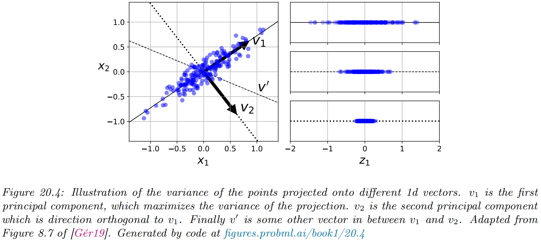
Optimal weight vector maximizes the variance of the projected data

• An interesting observation:
  $$\mathbb{E}\left[z_{n 1}\right]=\mathbb{E}\left[\boldsymbol{x}_{n}^{\top} \boldsymbol{w}_{1}\right]=\mathbb{E}\left[\boldsymbol{x}_{n}\right]^{\top} \boldsymbol{w}_{1}=0$$

• The variance of the projected data is：
  $$\mathbb{V}\left[\tilde{\mathbf{z}}_{1}\right]=\mathbb{E}\left[\tilde{\mathbf{z}}_{1}^{2}\right]-\left(\mathbb{E}\left[\tilde{\mathbf{z}}_{1}\right]\right)^{2}=\frac{1}{N} \sum_{n=1}^{N} z_{n 1}^{2}-0=-\mathcal{L}\left(\boldsymbol{w}_{1}\right)+\text { const }$$

• conclusion: minimizing the reconstruction error is equivalent to maximizing the variance of the projected data:
  $$\arg \min _{\boldsymbol{w}_{1}} \mathcal{L}\left(\boldsymbol{w}_{1}\right)=\arg \max _{\boldsymbol{w}_{1}} \mathbb{V}\left[\tilde{\mathbf{z}}_{1}\left(\boldsymbol{w}_{1}\right)\right]$$

• PCA finds the directions of maximal variance:

Induction step

Now let us find another direction $\boldsymbol{w}_{2}$ to further minimize the reconstruction error, subject to $\boldsymbol{w}_{1}^{\top} \boldsymbol{w}_{2}=0$ and $\boldsymbol{w}_{2}^{\top} \boldsymbol{w}_{2}=1$. The error is
$$\mathcal{L}\left(\boldsymbol{w}_{1}, \tilde{\mathbf{z}}_{1}, \boldsymbol{w}_{2}, \tilde{\mathbf{z}}_{2}\right)=\frac{1}{N} \sum_{n=1}^{N}\left\|\boldsymbol{x}_{n}-z_{n 1} \boldsymbol{w}_{1}-z_{n 2} \boldsymbol{w}_{2}\right\|^{2}$$

Computational issues

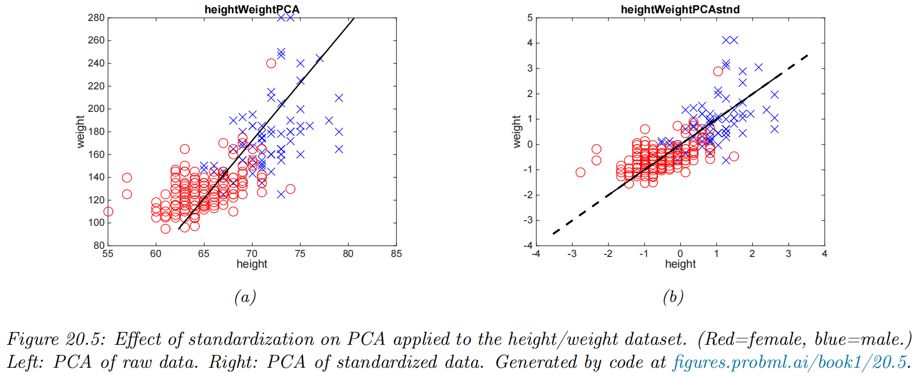
Covariance matrix vs correlation matrix

• better to use the correlation matrix instead of the covariance matrix

Dealing with high-dimensional data

• Finding eigenvectors of the $N \times N$ Gram matrix $\mathbf{X X}^{\top}$ is easier than $\mathbf{X}^{\top} \mathbf{X}$.

• let $\mathbf{U}$ be an orthogonal matrix containing the eigenvectors of $\mathbf{X} \mathbf{X}^{\top}$ with corresponding eigenvalues in $\boldsymbol{\Lambda}$.

$$\left(\mathbf{X X}^{\top}\right) \mathbf{U}=\mathbf{U} \boldsymbol{\Lambda}$$

• Pre-multiplying by $\mathbf{X}^{\top}$ gives
  $$\left(\mathbf{X}^{\top} \mathbf{X}\right)\left(\mathbf{X}^{\top} \mathbf{U}\right)=\left(\mathbf{X}^{\top} \mathbf{U}\right) \boldsymbol{\Lambda}$$

• the eigenvectors of $\mathbf{X}^{\top} \mathbf{X}$ are $\mathbf{V}=\mathbf{X}^{\top} \mathbf{U}$, with eigenvalues given by $\boldsymbol{\Lambda}$ as before.

• The normalized eigenvectors are given by
  $$\mathbf{V}=\mathbf{X}^{\top} \mathbf{U} \mathbf{\Lambda}^{-\frac{1}{2}}$$

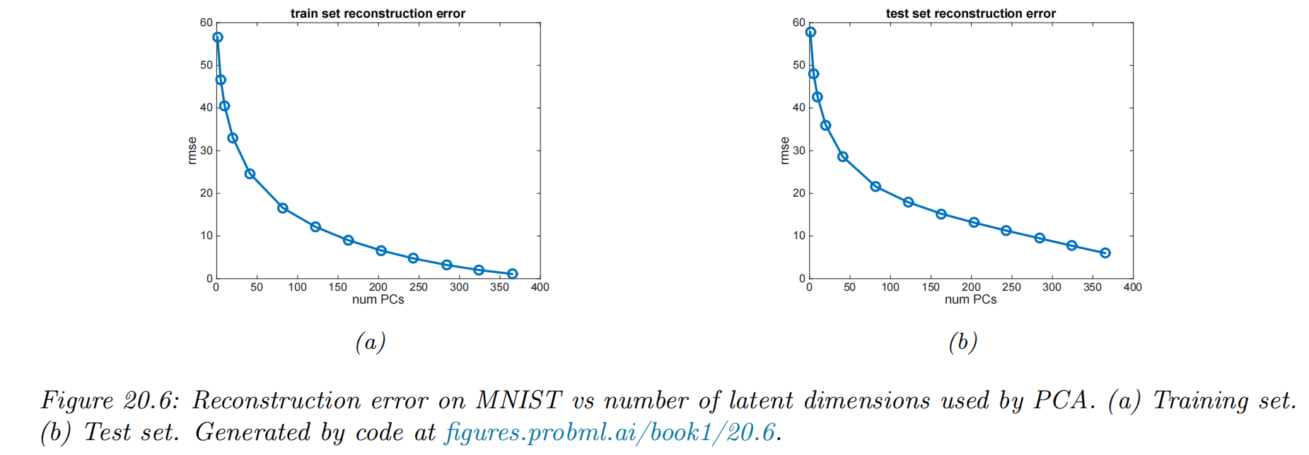
Choosing the number of latent dimensions

Reconstruction error

$$\mathcal{L}_L\frac{1}{|\mathcal{D}|}\sum_{n\in\mathcal{D}}\|x_n-\hat{x}_n\|^2$$

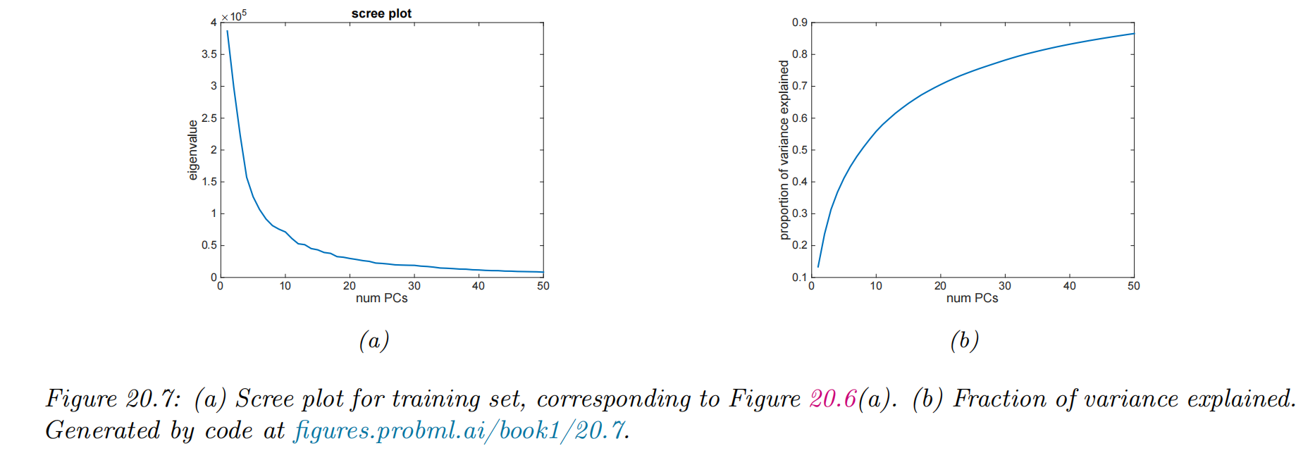
Scree plots

$$\mathcal{L}_\lambda=\sum_{j=L+1}^D\lambda_j$$

$$F_L=\frac{\sum_{j=1}^L\lambda_j}{\sum_{j'=1}^{L^{\max}}\lambda_j'}$$

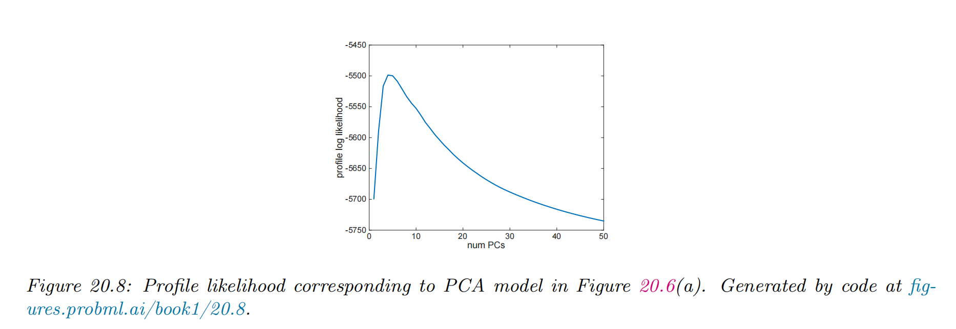
Profile likelihood

$$\begin{aligned} \mu_{1}(L) &=\frac{\sum_{k \leq L} \lambda_{k}}{L} \\ \mu_{2}(L) &=\frac{\sum_{k>L} \lambda_{k}}{L^{\max }-L} \\ \sigma^{2}(L) &=\frac{\sum_{k \leq L}\left(\lambda_{k}-\mu_{1}(L)\right)^{2}+\sum_{k>L}\left(\lambda_{k}-\mu_{2}(L)\right)^{2}}{L^{\max }} \end{aligned}$$
We can then evaluate the profile log likelihood
$$\ell(L)=\sum_{k=1}^{L} \log \mathcal{N}\left(\lambda_{k} \mid \mu_{1}(L), \sigma^{2}(L)\right)+\sum_{k=L+1}^{L^{\max }} \log \mathcal{N}\left(\lambda_{k} \mid \mu_{2}(L), \sigma^{2}(L)\right)$$

$L^{*}=\operatorname{argmax} \ell(L)$

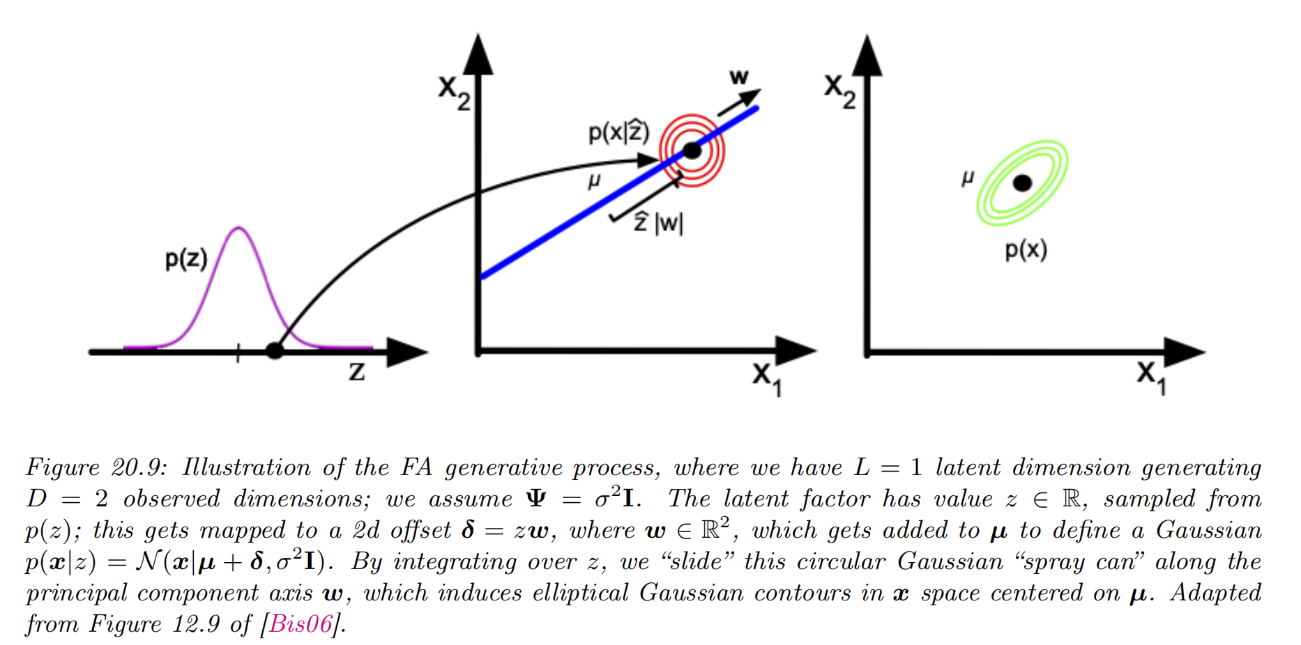
Factor analysis *

Generative model

• Factor analysis corresponds to the following linear-Gaussian latent variable generative model:
  $$\begin{aligned} p(\boldsymbol{z}) &=\mathcal{N}\left(\boldsymbol{z} \mid \boldsymbol{\mu}_{0}, \boldsymbol{\Sigma}_{0}\right) \\ p(\boldsymbol{x} \mid \boldsymbol{z}, \boldsymbol{\theta}) &=\mathcal{N}(\boldsymbol{x} \mid \mathbf{W} \boldsymbol{z}+\boldsymbol{\mu}, \boldsymbol{\Psi}) \end{aligned}$$
  where $\mathbf{W}$ is a $D \times L$ matrix, known as the factor loading matrix, and $\boldsymbol{\Psi}$ is a diagonal $D \times D$ covariance matrix.

• FA can be thought of as a low-rank version of a Gaussian distribution.
  $$\begin{aligned} p(\boldsymbol{x} \mid \boldsymbol{\theta}) &=\int \mathcal{N}(\boldsymbol{x} \mid \mathbf{W} \boldsymbol{z}+\boldsymbol{\mu}, \boldsymbol{\Psi}) \mathcal{N}\left(\boldsymbol{z} \mid \boldsymbol{\mu}_{0}, \boldsymbol{\Sigma}_{0}\right) d \boldsymbol{z} \\ &=\mathcal{N}\left(\boldsymbol{x} \mid \mathbf{W} \boldsymbol{\mu}_{0}+\boldsymbol{\mu}, \boldsymbol{\Psi}+\mathbf{W} \boldsymbol{\Sigma}_{0} \mathbf{W}^{\top}\right) \end{aligned}$$

  • $\mathbb{E}[\boldsymbol{x}]=\mathbf{W} \boldsymbol{\mu}_{0}+\boldsymbol{\mu}$
  • $\operatorname{Cov}[\boldsymbol{x}]=\mathbf{W \operatorname { C o v }}[\boldsymbol{z}] \mathbf{W}^{\boldsymbol{\top}}+\boldsymbol{\Psi}=\mathbf{W} \boldsymbol{\Sigma}_{0} \mathbf{W}^{\boldsymbol{\top}}+\boldsymbol{\Psi}$.

• a simplification:
  $$\begin{aligned} p(\boldsymbol{z}) &=\mathcal{N}(\boldsymbol{z} \mid \mathbf{0}, \mathbf{I}) \\ p(\boldsymbol{x} \mid \boldsymbol{z}) &=\mathcal{N}(\boldsymbol{x} \mid \mathbf{W} \boldsymbol{z}+\boldsymbol{\mu}, \boldsymbol{\Psi}) \\ p(\boldsymbol{x}) &=\mathcal{N}\left(\boldsymbol{x} \mid \boldsymbol{\mu}, \mathbf{W} \mathbf{W}^{\top}+\boldsymbol{\Psi}\right) \end{aligned}$$

• In general, FA approximates the covariance matrix of the visible vector using a low-rank decomposition:
  $$\mathbf{C}=\operatorname{Cov}[\boldsymbol{x}]=\mathbf{W} \mathbf{W}^{\top}+\boldsymbol{\Psi}$$

• We can estimate the parameters of an FA model using EM.

Probabilistic PCA

• a special case
  • $\mathbf{W}$ has orthonormal columns, $\boldsymbol{\Psi}=\sigma^{2} \mathbf{I}$ and $\boldsymbol{\mu}=\mathbf{0}$.
  • This model is called probabilistic principal components analysis (PPCA), or sensible PCA.
• The marginal distribution on the visible variables has the form
  $$p(\boldsymbol{x} \mid \boldsymbol{\theta})=\int \mathcal{N}\left(\boldsymbol{x} \mid \mathbf{W} \boldsymbol{z}, \sigma^{2} \mathbf{I}\right) \mathcal{N}(\boldsymbol{z} \mid \mathbf{0}, \mathbf{I}) d \boldsymbol{z}=\mathcal{N}(\boldsymbol{x} \mid \boldsymbol{\mu}, \mathbf{C})$$
  where
  $$\mathbf{C}=\mathbf{W} \mathbf{W}^{\top}+\sigma^{2} \mathbf{I}$$
• The log likelihood for PPCA is given by
  $$\log p\left(\mathbf{X} \mid \boldsymbol{\mu}, \mathbf{W}, \sigma^{2}\right)=-\frac{N D}{2} \log (2 \pi)-\frac{N}{2} \log |\mathbf{C}|-\frac{1}{2} \sum_{n=1}^{N}\left(\boldsymbol{x}_{n}-\boldsymbol{\mu}\right)^{\top} \mathbf{C}^{-1}\left(\boldsymbol{x}_{n}-\boldsymbol{\mu}\right)$$
• The MLE for $\boldsymbol{\mu}$ is $\overline{\boldsymbol{x}}$. Plugging in gives
  $$\log p\left(\mathbf{X} \mid \boldsymbol{\mu}, \mathbf{W}, \sigma^{2}\right)=-\frac{N}{2}\left[D \log (2 \pi)+\log |\mathbf{C}|+\operatorname{tr}\left(\mathbf{C}^{-1} \mathbf{S}\right)\right]$$
  where $\mathbf{S}=\frac{1}{N} \sum_{n=1}^{N}\left(\boldsymbol{x}_{n}-\overline{\boldsymbol{x}}\right)\left(\boldsymbol{x}_{n}-\overline{\boldsymbol{x}}\right)^{\top}$ is the empirical covariance matrix.
  In [TB99; Row97] they show that the maximum of this objective must satisfy
  $$\mathbf{W}=\mathbf{U}_{L}\left(\mathbf{L}_{L}-\sigma^{2} \mathbf{I}\right)^{\frac{1}{2}} \mathbf{R}$$

where $\mathbf{U}_{L}$ is a $D \times L$ matrix whose columns are given by the $L$ eigenvectors of $\mathbf{S}$ with largest eigenvalues, $\mathbf{L}_{L}$ is the $L \times L$ diagonal matrix of eigenvalues, and $\mathbf{R}$ is an arbitrary $L \times L$ orthogonal matrix, which (WLOG) we can take to be $\mathbf{R}=\mathbf{I}$. In the noise-free limit, where $\sigma^{2}=0$, we see that $\mathbf{W}_{\text {mle }}=\mathbf{U}_{L} \mathbf{L}_{L}^{\frac{1}{2}}$, which is proportional to the $\mathrm{PCA}$ solution.

• The MLE for the observation variance is
  $$\sigma^{2}=\frac{1}{D-L} \sum_{i=L+1}^{D} \lambda_{i}$$
  which is the average distortion associated with the discarded dimensions. If $L=D$, then the estimated noise is 0 , since the model collapses to $\boldsymbol{z}=\boldsymbol{x}$.

• To use PPCA as an alternative to $\mathrm{PCA}$, we need to compute the posterior mean $\mathbb{E}[\boldsymbol{z} \mid \boldsymbol{x}]$, which is the equivalent of the encoder model. Using Bayes rule for Gaussians we have
  $$p(\boldsymbol{z} \mid \boldsymbol{x})=\mathcal{N}\left(\boldsymbol{z} \mid \mathbf{M}^{-1} \mathbf{W}^{\top}(\boldsymbol{x}-\boldsymbol{\mu}), \sigma^{2} \mathbf{M}^{-1}\right)$$
  where $\mathbf{M}$ is defined in Equation (20.48). In the $\sigma^{2}=0$ limit, the posterior mean using the MLE parameters becomes
  $$\mathbb{E}[\boldsymbol{z} \mid \boldsymbol{x}]=\left(\mathbf{W}^{\top} \mathbf{W}\right)^{-1} \mathbf{W}^{\top}(\boldsymbol{x}-\overline{\boldsymbol{x}})$$
  which is the orthogonal projection of the data into the latent space, as in standard PCA.

Factor analysis models for paired data

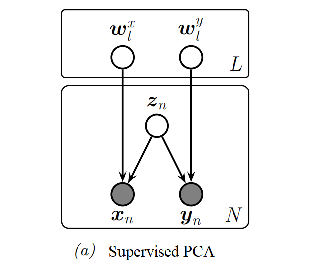
Supervised PCA

• model the joint $p(\boldsymbol{x}, \boldsymbol{y})$ using a shared low-dimensional representation using the following linear Gaussian model:
  $$\begin{aligned} p\left(\boldsymbol{z}_{n}\right) &=\mathcal{N}\left(\boldsymbol{z}_{n} \mid \mathbf{0}, \mathbf{I}_{L}\right) \\ p\left(\boldsymbol{x}_{n} \mid \boldsymbol{z}_{n}, \boldsymbol{\theta}\right) &=\mathcal{N}\left(\boldsymbol{x}_{n} \mid \mathbf{W}_{x} \boldsymbol{z}_{n}, \sigma_{x}^{2} \mathbf{I}_{D_{x}}\right) \\ p\left(\boldsymbol{y}_{n} \mid \boldsymbol{z}_{n}, \boldsymbol{\theta}\right) &=\mathcal{N}\left(\boldsymbol{y}_{n} \mid \mathbf{W}_{y} \boldsymbol{z}_{n}, \sigma_{y}^{2} \mathbf{I}_{D_{y}}\right) \end{aligned}$$

• $\boldsymbol{z}_{n}$ is a shared latent subspace, that captures features that $\boldsymbol{x}_{n}$ and $\boldsymbol{y}_{n}$ have in common.

• The variance terms $\sigma_{x}$ and $\sigma_{y}$ control how much emphasis the model puts on the two different signals.

• If we put a prior on the parameters $\boldsymbol{\theta}=\left(\mathbf{W}_{x}, \mathbf{W}_{y}, \sigma_{x}, \sigma_{y}\right)$, we recover the Bayesian factor regression model.

• We can marginalize out $\boldsymbol{z}_{n}$ to get $p\left(\boldsymbol{y}_{n} \mid \boldsymbol{x}_{n}\right)$. If $\boldsymbol{y}_{n}$ is a scalar, this becomes
  $$\begin{aligned} p\left(y_{n} \mid \boldsymbol{x}_{n}, \boldsymbol{\theta}\right) &=\mathcal{N}\left(y_{n} \mid \boldsymbol{x}_{n}^{\top} \boldsymbol{v}, \boldsymbol{w}_{y}^{\top} \mathbf{C} \boldsymbol{w}_{y}+\sigma_{y}^{2}\right) \\ \mathbf{C} &=\left(\mathbf{I}+\sigma_{x}^{-2} \mathbf{W}_{x}^{\top} \mathbf{W}_{x}\right)^{-1} \\ \boldsymbol{v} &=\sigma_{x}^{-2} \mathbf{W}_{x} \mathbf{C} \boldsymbol{w}_{y} \end{aligned}$$

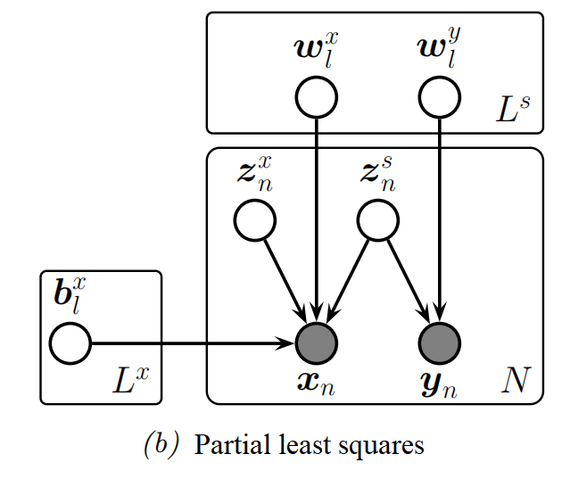
Partial least squares

• Another way to improve the predictive performance in supervised tasks is to allow the inputs $\boldsymbol{x}$ to have their own "private" noise source that is independent on the target variable

• introducing an extra latent variable $\boldsymbol{z}_{n}^{x}$ just for the inputs, that is different from $\boldsymbol{z}_{n}^{s}$ that is the shared bottleneck between $\boldsymbol{x}_{n}$ and $\boldsymbol{y}_{n}$.

• In the Gaussian case, the overall model has the form
  $$\begin{aligned} p\left(\boldsymbol{z}_{n}\right) &=\mathcal{N}\left(\boldsymbol{z}_{n}^{s} \mid \mathbf{0}, \mathbf{I}\right) \mathcal{N}\left(\boldsymbol{z}_{n}^{x} \mid \mathbf{0}, \mathbf{I}\right) \\ p\left(\boldsymbol{x}_{n} \mid \boldsymbol{z}_{n}, \boldsymbol{\theta}\right) &=\mathcal{N}\left(\boldsymbol{x}_{n} \mid \mathbf{W}_{x} \boldsymbol{z}_{n}^{s}+\mathbf{B}_{x} \boldsymbol{z}_{n}^{x}, \sigma_{x}^{2} \mathbf{I}\right) \\ p\left(\boldsymbol{y}_{n} \mid \boldsymbol{z}_{n}, \boldsymbol{\theta}\right) &=\mathcal{N}\left(\boldsymbol{y}_{n} \mid \mathbf{W}_{y} \boldsymbol{z}_{n}^{s}, \sigma_{y}^{2} \mathbf{I}\right) \end{aligned}$$

• MLE for $\boldsymbol{\theta}$ in this model is equivalent to the technique of partial least squares (PLS).

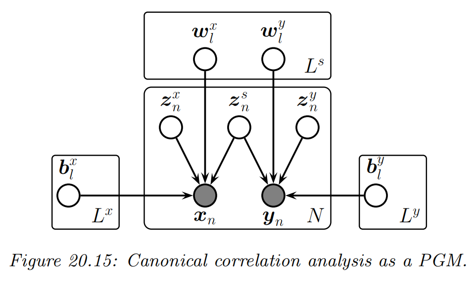
Canonical correlation analysis

• use a fully symmetric model:

  • a latent variable $\boldsymbol{z}^x_n$ just for $\boldsymbol{x}_n$
  • a latent variable $\boldsymbol{z}^y_n$ just for $\boldsymbol{y}_n$
  • a shared latent variable $\boldsymbol{z}^s_n$

• the Gaussian case:
  $$\begin{aligned} p\left(\boldsymbol{z}_{n}\right) &=\mathcal{N}\left(\boldsymbol{z}_{n}^{s} \mid \mathbf{0}, \mathbf{I}\right) \mathcal{N}\left(\boldsymbol{z}_{n}^{x} \mid \mathbf{0}, \mathbf{I}\right) \\ p\left(\boldsymbol{x}_{n} \mid \boldsymbol{z}_{n}, \boldsymbol{\theta}\right) &=\mathcal{N}\left(\boldsymbol{x}_{n} \mid \mathbf{W}_{x} \boldsymbol{z}_{n}^{s}+\mathbf{B}_{x} \boldsymbol{z}_{n}^{x}, \sigma_{x}^{2} \mathbf{I}\right) \\ p\left(\boldsymbol{y}_{n} \mid \boldsymbol{z}_{n}, \boldsymbol{\theta}\right) &=\mathcal{N}\left(\boldsymbol{y}_{n} \mid \mathbf{W}_{y} \boldsymbol{z}_{n}^{s}+\mathbf{B}_{y} \boldsymbol{z}_{n}^{y}, \sigma_{y}^{2} \mathbf{I}\right) \end{aligned}$$
  where $\mathbf{W}_{x}$ and $\mathbf{W}_{y}$ are $L^{s} \times D$ dimensional, $\mathbf{V}_{x}$ is $L^{x} \times D$ dimensional, and $\mathbf{V}_{y}$ is $L^{y} \times D$ dimensional.

• marginalizing out all the latent variables (where we assume $\sigma_{x}=\sigma_{y}=\sigma$ ):
  $$p\left(\boldsymbol{x}_{n}, \boldsymbol{y}_{n}\right)=\int d \boldsymbol{z}_{n} p\left(\boldsymbol{z}_{n}\right) p\left(\boldsymbol{x}_{n}, \boldsymbol{y}_{n} \mid \boldsymbol{z}_{n}\right)=\mathcal{N}\left(\boldsymbol{x}_{n}, \boldsymbol{y}_{n} \mid \boldsymbol{\mu}, \mathbf{W} \mathbf{W}^{\boldsymbol{\top}}+\sigma^{2} \mathbf{I}\right)$$

  where $\boldsymbol{\mu}=\left(\boldsymbol{\mu}_{x} ; \boldsymbol{\mu}_{y}\right)$, and $\mathbf{W}=\left[\mathbf{W}_{x} ; \mathbf{W}_{y}\right]$.

• Thus the induced covariance is the following low rank matrix:
  $$\mathbf{W} \mathbf{W}^{\top}=\left(\begin{array}{ll}\mathbf{W}_{x} \mathbf{W}_{x}^{\top} & \mathbf{W}_{x} \mathbf{W}_{y}^{\top} \\ \mathbf{W}_{y} \mathbf{W}_{y}^{\top} & \mathbf{W}_{y} \mathbf{W}_{y}^{\top}\end{array}\right)$$

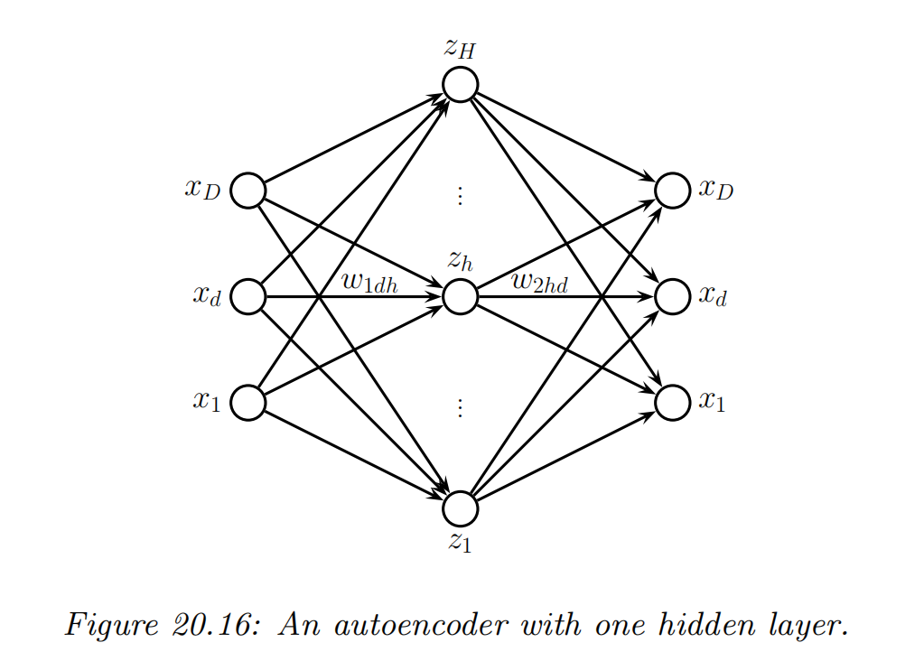
Autoencoders

• recall what we learned from PCA
  • Encoder: $f_e:\boldsymbol{x}\rightarrow\boldsymbol{z}$
  • Decoder: $f_d:\boldsymbol{z}\rightarrow\boldsymbol{x}$
  • The overall reconstruction function: $r(\boldsymbol{x})=f_d(f_e(\boldsymbol{x}))$
  • loss function: $\mathcal{L}(\boldsymbol{\theta})=\|r(\boldsymbol{x})-\boldsymbol{x}\|^2_2$ or $\mathcal{L}(\boldsymbol{\theta})=-\log p(\boldsymbol{x}|r(\boldsymbol{x}))$
• Autoencoder: the encoder and decoder are nonlinear mappings implemented by neural networks.
• Bottleneck: the hidden units in the middle (as a low-dimensional bottleneck) between the input and its reconstruction.