L01 Introduction of Machine Learning

Materials are adopted from "Murphy, Kevin P. Probabilistic machine learning: an introduction. MIT press, 2022.". This handout is only for teaching. DO NOT DISTRIBUTE.

What is ML

• Definition of ML

  A computer program is said to learn from experience $E$ with respect to some class of tasks $T$, and performance measure $P$, if its performance at tasks in $T$, as measured by $P$, improves with experience $E$.

  --Tom Mitchell

• The probabilistic approach

  • treat all unknown quantities as random variables
  • it is the optimal approach to decision making under uncertainty

  Almost all of machine learning can be viewed in probabilistic terms, making probabilistic thinking fundamental. It is, of course, not the only view. But it is through this view that we can connect what we do in machine learning to every other computational science, whether that be in stochastic optimisation, control theory, operations research, econometrics, information theory, statistical physics or bio-statistics. For this reason alone, mastery of probabilistic thinking is essential.

  ---Shakir Mohamed, DeepMind

• Machine Learning vs. Statistic Approaches

  • Statistical approaches rely on foundational assumptions and explicit models of structure, such as observed samples that are assumed to be drawn from a specified underlying probability distribution.
  • Machine learning seeks to extract knowledge from large amounts of data with no such restrictions -- “find the pattern, apply the pattern.”

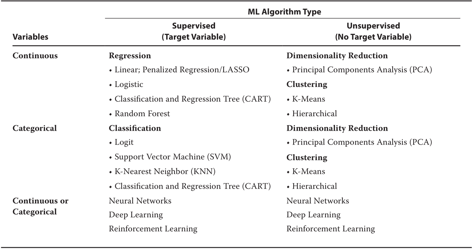
• Supervised Learning vs. Unsupervised Learning

  • Supervised learning involves ML algorithms that infer patterns between a set of inputs (the $X$’s) and the desired output ($Y$) with a labeled data set.
  • Unsupervised learning is machine learning that does not make use of labeled data. In unsupervised learning, inputs ($X$’s) are used for analysis without any target ($Y$) being supplied. The algorithm seeks to discover structure within the data themselves. Two important types of problems in unsupervised learning are dimension reduction and clustering.

• Deep Learning and Reinforcement Learning

  • In deep learning, sophisticated algorithms address highly complex tasks, such as image classification, face recognition, speech recognition, and natural language processing.
  • reinforcement learning, a computer learns from interacting with itself (or data generated by the same algorithm).
  • Neural networks (NNs, also called artificial neural networks, or ANNs) include highly flexible ML algorithms that have been successfully applied to a variety of tasks characterized by non-linearities and interactions among features.
  • Besides being commonly used for classification and regression, neural networks are also the foundation for deep learning and reinforcement learning, which can be either supervised or unsupervised.

Supervised Learning

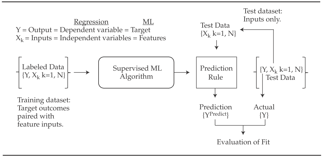
• Definition
  • The task $T$ is to learn a mapping $f$ from inputs $\mathbf{x}\in\mathcal{X}$ to outputs $y\in\mathcal{Y}$
  • The inputs $\mathbf{x}$ are also called the features, covariates, or predictors
  • The outputs $y$ are also called the label, target, or response
  • The experince $E$ is the training set $\mathcal{D}=\{(x_n,y_n)\}_{n=1}^N$

Classification

classification problem

• the output space is a set of $C$ unordered and mutually exclusive labels known as classes, $\mathcal{Y} = \{1, 2, . . . , C\}$.
• The problem is also called pattern recognition.
• binary classification: just two classes, often denoted by
  • $y \in\{0, 1\}$
  • $y \in\{−1, +1\}$

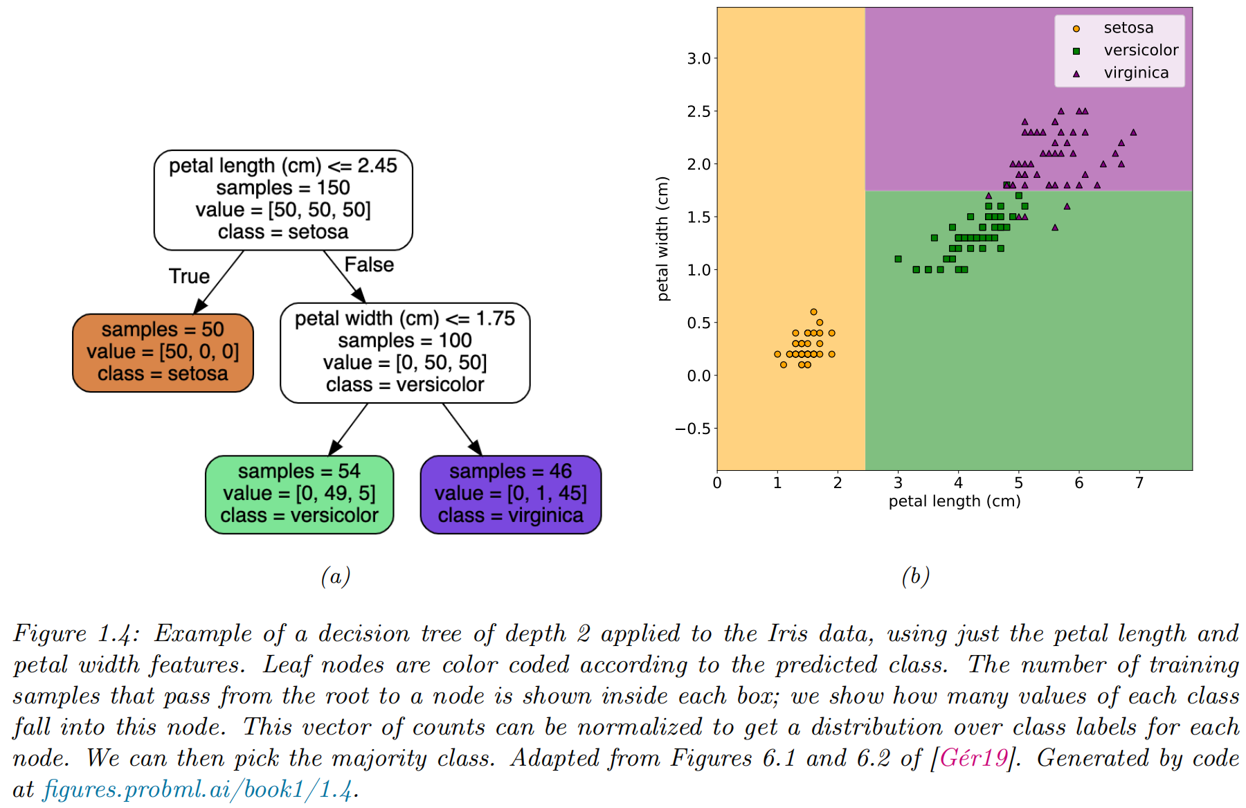
Example: classifying Iris flowers

Iris Flowers Classification

Image Classification

Exploratory data analysis

• exploratory data analysis: see if there are any obvious patterns
• tabular data with a small number of features: pair plot
• higher-dimensional data: dimension reduction first and then to visualize the data in 2d or 3d

Learning a classifier

• decision rule via a 1 dimensional (1d) decision boundary
  $$f(\mathbf{x};\theta)=\left\{\begin{array}{l}\text{Setosa if petal lenth}<2.45\\\text{Versicolor or Virginica otherwise}\end{array}\right.$$

• decision tree a more sophisticated decision rule involves a 2d decision surface

Empirical risk minimization

• misclassification rate on the training set:
  $$\mathcal{L}(\theta)=\frac{1}{N}\sum_{n=1}^N\mathbb{I}(y_n\neq f(x_n;\theta))$$
• loss function: $l(y,\hat{y})$
• empirical risk: e the average loss of the predictor on the training set
  $$\mathcal{L}(\theta)=\frac{1}{N}\sum_{n=1}^Nl(y_n,f(x_n;\theta))$$
• model fitting / training via empirical risk minimization
  $$\hat{\theta}=\argmin_\theta\mathcal{L}(\theta)=\argmin_\theta\frac{1}{N}\sum_{n=1}^Nl(y_n,f(x_n;\theta))$$

Uncertainty

We must avoid] false confidence bred from an ignorance of the probabilistic nature of the world, from a desire to see black and white where we should rightly see gray.

--- Immanuel Kant, as paraphrased by Maria Konnikova

• Two types of uncertainties
  • epistemic uncertainty or model uncertainty: due to
    lack of knowledge of the input-output mapping
  • aleatoric uncertainty or data uncertainty: due to intrinsic (irreducible) stochasticity in the mapping
• We can capture our uncertainty using the following conditional probability distribution:
  $$p(y=c|\mathbf{x};\theta)=f_c(\mathbf{x};\theta)$$

Maximum likelihood estimation

• likelihood function: $p(y \mid f(\boldsymbol{x} ; \boldsymbol{\theta}))$

• log likelihood function
  $$\ell(y, f(\boldsymbol{x} ; \boldsymbol{\theta}))=-\log p(y \mid f(\boldsymbol{x} ; \boldsymbol{\theta}))$$

• Negative Log Likelihood: The average negative $\log$ probability of the training set.
  $$\operatorname{NLL}(\boldsymbol{\theta})=-\frac{1}{N} \sum_{n=1}^{N} \log p\left(y_{n} \mid f\left(\boldsymbol{x}_{n} ; \boldsymbol{\theta}\right)\right)$$

• the maximum likelihood estimate (MLE):
  $$\hat{\boldsymbol{\theta}}_{\mathrm{mle}}=\underset{\boldsymbol{\theta}}{\operatorname{argmin}} \mathrm{NLL}(\boldsymbol{\theta})$$

Regression

regression problem

• the output space: $y\in\mathcal{Y} = \mathbb{R}$.
• loss function: quadratic loss, or $\ell_2$ loss:
  $$\ell(y,\hat{y})=(y-\hat{y})^2$$
• mean squared error or MSE:
  $$\operatorname{MSE}(\boldsymbol{\theta})=\frac{1}{N}\sum_{n=1}^N(y_n-f(\boldsymbol{x}_n;\boldsymbol{\theta}))^2$$
• An Example
  • Uncertainty: Guassian / Normal
    $$\mathcal{N}(y|\mu,\sigma^2)\triangleq\frac{1}{\sqrt{2\pi\sigma^2}}e^{-\frac{1}{2\sigma^2}(y-\mu)^2}$$
  • the conditional dist
    $$p(y|\boldsymbol{x};\boldsymbol{\theta})=\mathcal{N}(y|f(\boldsymbol{x};\boldsymbol{\theta}),\sigma^2)$$
  • NLL
    $$\begin{array}{lll}\operatorname{NLL}(\boldsymbol{\theta})&=&-\frac{1}{N} \sum_{n=1}^{N} \log\left[\left(\frac{1}{2\pi\sigma^2}\right)^{\frac{1}{2}}\exp\left(-\frac{1}{2\sigma^2}(y_n-f(\boldsymbol{x}_n;\boldsymbol{\theta}))^2\right)\right]\\ &=&-\frac{1}{2\sigma^2}\operatorname{MSE}(\boldsymbol{\theta})+\text{const}\end{array}$$

(simple) Linear regression

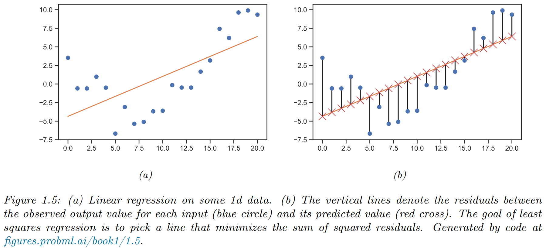
• functional form of model:
  $$f(x;\boldsymbol{\theta})=b+wx$$
• parameters: $\boldsymbol{\theta}=(w,b)$
• least square estimator:
  $$\hat{\boldsymbol{\theta}}=\argmin_{\boldsymbol{\theta}}\operatorname{MSE}(\boldsymbol{\theta})$$

Polynomial regression

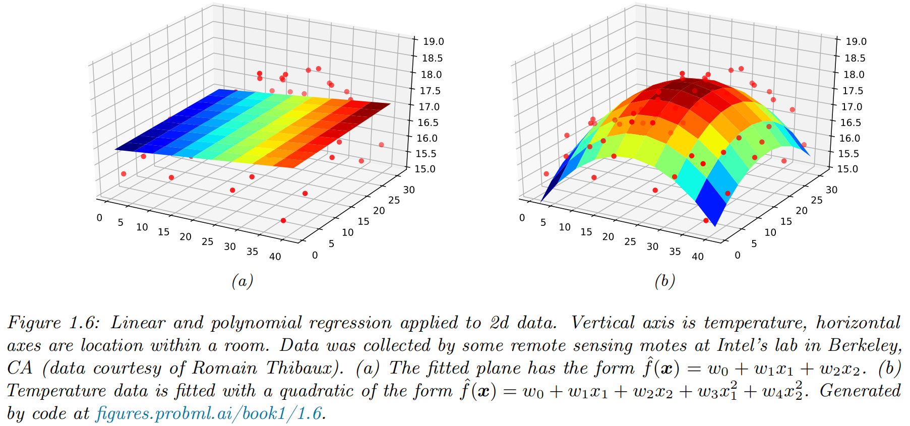
• functional form of model:
  $$f(x;\boldsymbol{\theta})=\boldsymbol{w}^{\top}\phi(x)$$
• feature preprocessing, or feature engineering
  $$\phi(x)=[1,x,x^2,\dots,x^D]$$

Deep neural networks

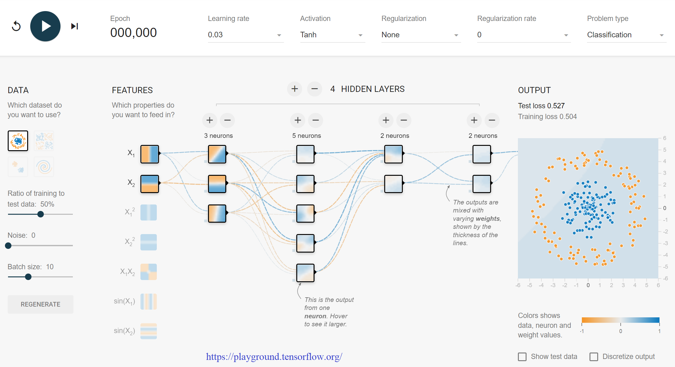
• deep neural networks (DNN): a stack of L nested functions:
  $$f(\boldsymbol{x};\boldsymbol{\theta})=f_L(f_{L-1}(\cdots f_1(\boldsymbol{x})\cdots))$$
• the function at layer $\ell$: $f_{\ell}(\boldsymbol{x};\boldsymbol{\theta}_{\ell})$
  • the final layer:
    $$f_L(\boldsymbol{x})=\boldsymbol{w}^{\top}f_{1:L-1}(\boldsymbol{x})$$
  • the learned feature extractor: $f_{1:L-1}(\boldsymbol{x})$

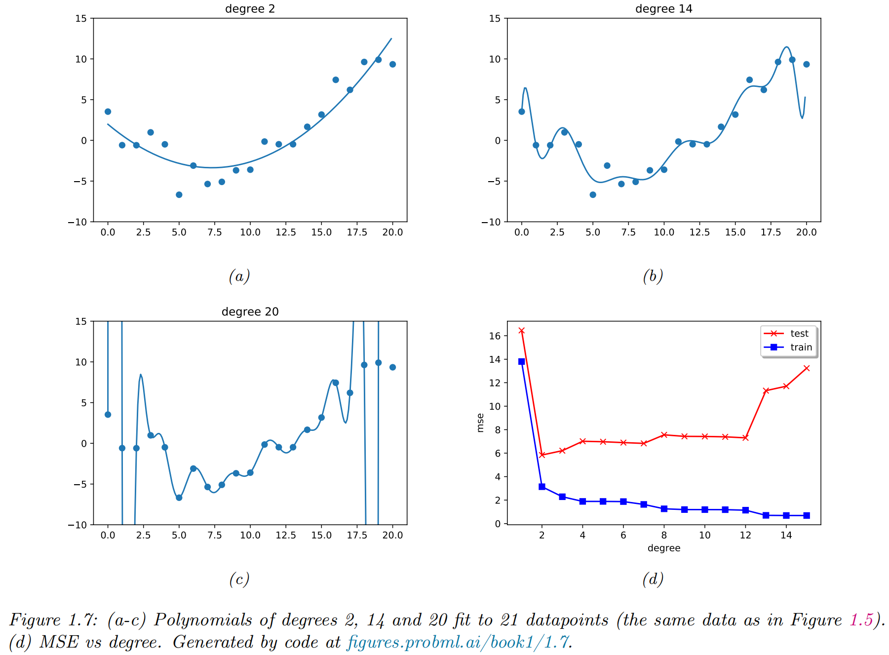
Overfitting and generalization

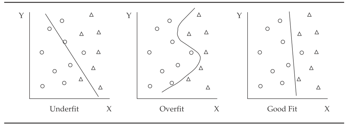
• Underfitting means the model does not capture the relationships in the data.

• Overfitting means the model begins to incorporate noise coming from quirks or spurious correlations

  • it mistakes randomness for patterns and relationships
  • memorized the data, rather than learned from it
  • high noise levels in the data and too much complexity in the model
  • complexity refers to the number of features, terms, or branches in the model and to whether the model is linear or non-linear (non-linear is more complex).

• empirical risk
  $$\mathcal{L}\left(\boldsymbol{\theta} ; \mathcal{D}_{\text {train }}\right)=\frac{1}{\left|\mathcal{D}_{\text {train }}\right|} \sum_{(\boldsymbol{x}, \boldsymbol{y}) \in \mathcal{D}_{\text {train }}} \ell(\boldsymbol{y}, f(\boldsymbol{x} ; \boldsymbol{\theta}))$$

• population risk
  $$\mathcal{L}(\boldsymbol{\theta};p^*)\triangleq\mathbb{E}_{p^*_{(\boldsymbol{x},\boldsymbol{y})}}[\ell(\boldsymbol{y},f(\boldsymbol{x};\boldsymbol{\theta}))]$$

• generalization gap: $\mathcal{L}(\boldsymbol{\theta};p^*)-\mathcal{L}\left(\boldsymbol{\theta} ; \mathcal{D}_{\text {train }}\right)$

• test risk
  $$\mathcal{L}\left(\boldsymbol{\theta} ; \mathcal{D}_{\text {test }}\right)=\frac{1}{\left|\mathcal{D}_{\text {test }}\right|} \sum_{(\boldsymbol{x}, \boldsymbol{y}) \in \mathcal{D}_{\text {test }}} \ell(\boldsymbol{y}, f(\boldsymbol{x} ; \boldsymbol{\theta}))$$

Evaluating ML Algorithm Performance Errors & Overfitting

• Data scientists decompose the total out-of-sample error into three sources:
  • Bias error, or the degree to which a model fits the training data. Algorithms with erroneous assumptions produce high bias with poor approximation, causing underfitting and high in-sample error.
  • Variance error, or how much the model's results change in response to new data from validation and test samples. Unstable models pick up noise and produce high variance, causing overfitting
  • Base error due to randomness in the data.

learning curve

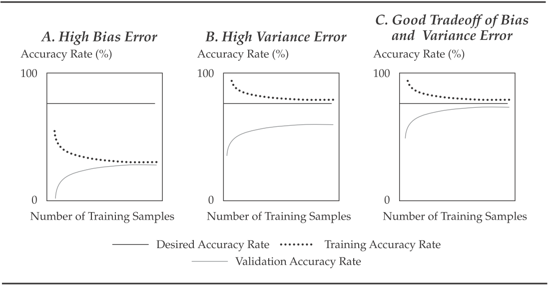
• A learning curve plots the accuracy rate (= 1 – error rate) in the validation or test samples (i.e., out-of-sample) against the amount of data in the training sample

fitting curve

• A fitting curve, which shows in-and out-of-sample error rates ($E_\text{in}$ and $E_\text{out}$) on the $y$-axis plotted against model complexity on the $x$-axis

Evaluating ML Algorithm Performance: Preventing Overfitting in Supervised ML

• Two common guiding principles and two methods are used to reduce overfitting:

  • preventing the algorithm from getting too complex during selection and training (regularization)
  • proper data sampling achieved by using cross-validation

• K-fold cross-validation

  • data (excluding test sample and fresh data) are shuffled randomly and then are divided into k equal sub-samples
  • $k-1$ samples used as training samples and one sample used as a validation sample
  • $k$ is typically set at 5 or 10
  • This process is repeated $k$ times. The average of the $k$ validation errors (mean $E_\text{val}$) is taken as a reasonable estimate of the model's out-of-sample error ($E_\text{out}$)

• Leave-one-out cross-validation: $k=N$

No free lunch theorem

All models are wrong, but some models are useful.

--- George Box

• No free lunch theorem: There is no single best model that works optimally for all kinds of problems
• pick a suitable model
  • based on domain knowledge
  • trial and error
    • cross-validation
    • Bayesian methods selection techniques

Unsupervised learning

• unsupervised learning: “inputs” $\mathcal{D} = \{x_n : n = 1 : N\}$ without any corresponding “outputs” $y_n$.
• the task: fitting an unconditional model of the form $p(x)$

When we’re learning to see, nobody’s telling us what the right answers are — we just look. Every so often, your mother says “that’s a dog”, but that’s very little information. You’d be lucky if you got a few bits of information — even one bit per second — that way. The brain’s visual system has 1014 neural connections. And you only live for 109 seconds. So it’s no use learning one bit per second. You need more like 105 bits per second. And there’s only one place you can get that much information: from the input itself.

--- Geoffrey Hinton, 1996

Clustering

• finding clusters in data: partition the input into regions that contain “similar” points.

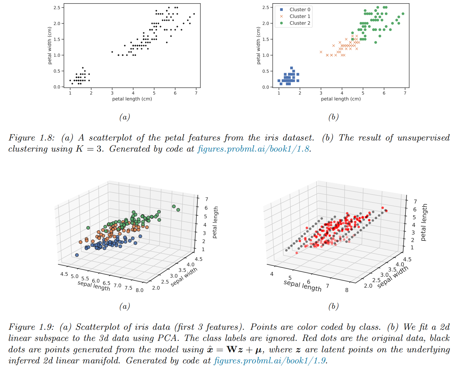
Discovering latent “factors of variation”

• Assume that each observed high-dimensional output $\boldsymbol{x}_n\in\mathbb{R}^D$ was generated by a set of hidden or unobserved low-dimensional latent factors $\boldsymbol{z}_n\in\mathbb{R}^K$.

• factor analysis (FA)
  $$p(\boldsymbol{x}_n|\boldsymbol{z}_n;\boldsymbol{\theta})=\mathcal{N}(\boldsymbol{x}_n|\boldsymbol{W}_n\boldsymbol{z}_n+\boldsymbol{\mu},\boldsymbol{\Sigma})$$

• principal components analysis (PCA): $\boldsymbol{\Sigma}=\sigma^2\boldsymbol{I}$

• nonlinear models: neural networks

Reinforcement learning

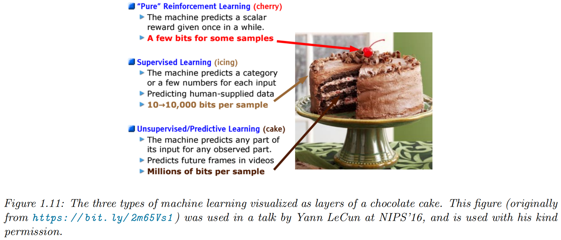
• online / dynamic version of machine learning
  • the system or agent has to learn how to interact
    with its environment
  • RL is closely related to the Markov Decision Process (MDP)

Markov Decision Process

The MDP is the sequence of random variables ($X_n$) which describes the stochastic evolution of the system states. Of course the distribution of ($X_n$) depends on the chosen actions.

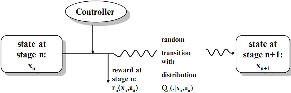
• $E$ denotes the state space of the system. A state $x\in E$ is the information which is available for the controller at time $n$. Given this information an action has to be selected.

• $A$ denotes the action space. Given a specific state $x\in E$ at time $n$, a certain subclass $D_n(x)\subset A$ of actions may only be admissible.

• $Q_n(B|x,a)$ is a stochastic transition kernel which gives the probability that the next state at time $n+1$ is in the set B if the current state is $x$ and action a is taken at time $n$.

• $r_n(x, a)$ gives the (discounted) one-stage reward of the system at time $n$ if the current state is $x$ and action a is taken

• $g_N(x)$ gives the (discounted) terminal reward of the system at the end of the planning horizon.

A control $\pi$ is a sequence of decision rules ($f_n$) with $f_n:E\rightarrow A$ where $f_n(x)\in D_n(x)$ determines for each possible state $x\in E$ the next action $f_n(x)$ at time $n$. Such a sequence $\pi=(f_n)$ is called policy or strategy. Formally the Markov Decision Problem is given by

$$V_0(x)=\sup_{\pi}\mathbb{E}_x^{\pi}\left[\sum_{k=0}^{N-1}r_k\left(X_k,f_k(X_k)\right)+g_N(X_N)\right],\text{ }x\in E.$$

• Types of MDP problems:

  • finite horizon ($N<\infty$) vs. infinite horizon ($N=\infty$)
  • complete state observation vs. partial state observation
  • problems with constraints vs. without constraints
  • total (discounted) cost criterion vs. average cost criterion

• Research questions:

  • Does an optimal policy exist?
  • Has it a particular form?
  • Can an optimal policy be computed efficiently?
  • Is it possible to derive properties of the optimal value function analytically?

Applications of MDP: Comsumption Problem

Suppose there is an investor with given initial capital. At the beginning of each of $N$ periods she can decide how much of the capital she consumes and how much she invests into a risky asset. The amount she consumes is evaluated by a utility function $U$ as well as the terminal wealth. The remaining capital is invested into a risky asset where we assume that the investor is small and thus not able to influence the asset price and the asset is liquid. How should she consume/invest in order to maximize the sum of her expected discounted utility?

Applications of MDP: Cash Balance or Inventory Problem

Imagine a company which tries to find the optimal level of cash over a finite number of $N$ periods. We assume that there is a random stochastic change in the cash reserve each period (due to withdrawal or earnings). Since the firm does not earn interest from the cash position, there are holding cost for the cash reserve if it is positive, but also interest (cost) in case it is negative. The cash reserve can be increased or decreased by the management at each decision epoch which implies transfer costs. What is the optimal cash balance policy?

Applications of MDP: Mean-Variance Problem

Consider a small investor who acts on a given financial market. Her aim is to choose among all portfolios which yield at least a certain expected return (benchmark) after $N$ periods, the one with smallest portfolio variance. What is the optimal investment strategy?

Applications of MDP: Dividend Problem in Risk Theory

Imagine we consider the risk reserve of an insurance company which earns some premia on the one hand but has to pay out possible claims on the other hand. At the beginning of each period the insurer can decide upon paying a dividend. A dividend can only be paid when the risk reserve at that time point is positive. Once the risk reserve got negative we say that the company is ruined and has to stop its business. Which dividend pay-out policy maximizes the expected discounted dividends until ruin?

Applications of MDP: Bandit Problem

Suppose we have two slot machines with unknown success probability $\theta_1$ and $\theta_2$. At each stage we have to choose one of the arms. We receive one Euro if the arm wins, else no cash flow appears. How should we play in order to maximize our expected total reward over $N$ trials?

Applications of MDP: Pricing of American Options

In order to find the fair price of an American option and its optimal exercise time, one has to solve an optimal stopping problem. In contrast to a European option the buyer of an American option can choose to exercise any time up to and including the expiration time. Such an optimal stopping problem can be solved in the framework of Markov Decision Processes.

Discussion

Statistical inference vs. Supervised machine learning

Property	Statistical inference	Supervised machine learning
Goal	Causal models with explanatory power	Prediction performance, often with limited explanatory power
Data	The data is generated by a model	The data generation process is unknown
Framework	Probabilistic	Algorithmic and Probabilistic
Expressibility	Typically linear	Non-linear
Model selection	Based on information criteria	Numerical optimization
Scalability	Limited to lower-dimensional data	Scales to high-dimensional input data
Robustness	Prone to over-fitting	Designed for out-of-sample performance
Diagnostics	Extensive	Limited

Financial Econometrics and Machine Learning

ML Algorithm Types

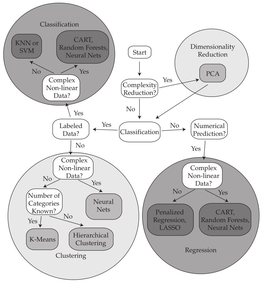
Selecting ML Algorithms

Useful Python Libraries

Popular Data Science Libraries in Python

Math Libraries

• Scipy
  
  
  
  

• Numpy
  
  
  

• Pandas
  
  
  

Statistical Libraries

• StatsModels
  
  
  

ML and Deep Learning

• scikit-learn
  
  
  

• TensorFlow
  
  
  

• PyTorch
  
  
  

• Theano

Decision Theory

Bayesian decision theory

Basics

The decision maker, or agent, has a set of possible actions, $\mathcal{A}$, to choose from. Each of these actions has costs and benefits, which will depend on the underlying state of nature $H\in\mathcal{H}$. We can encode this information into a loss function $\mathcal{l}(h, a)$, that specifies the loss we incur if we take action $a\in\mathcal{A}$ when the state of nature is $h\in\mathcal{H}$.

• The posterior expected loss or risk for each possible action:

$$R(a|\mathbf{x})=\mathbb{E}_{p(h|\mathbf{x})}[\mathcal{l}(h,a)]=\sum_{h\in\mathcal{H}}\mathcal{l}(h,a)p(h|\mathbf{x})$$

• The optimal policy (also called the Bayes estimator) specifies what action to take for each possible observation so as to minimize the risk:

$$\pi^*(\mathbf{x})=\argmin_{a\in\mathcal{A}}\mathbb{E}_{p(h|\mathbf{x})}[\mathcal{l}(h,a)]$$

• Let $U(h,a)=-l(h,a)$ be the utility function, then the optimal policy is as follows (maximum expected utility principle):

$$\pi^*(\mathbf{x})=\argmax_{a\in\mathcal{A}}\mathbb{E}_{p(h|\mathbf{x})}[U(h,a)]$$

Classification problems

We use Bayesian decision theory to decide the optimal class label to predict given an observed input $x\in X$.

Zero-one loss

Suppose the states of nature correspond to class labels, so $\mathcal{H} = \mathcal{Y} = \{1, . . . , C\}$. Furthermore, suppose the actions also correspond to class labels, so $\mathcal{A} = \mathcal{Y}$. In this setting, a very commonly used

• the zero-one loss $l_{01}(y^∗, \hat{y})=\mathbb{I}(y^*\neq\hat{y})$, defined as follows:

	$\hat{y}=0$	$\hat{y}=1$
$y^*=0$	$0$	$1$
$y^*=1$	$1$	$0$

• the posterior expected loss

$$R(\hat{y}|\mathbf{x})=p(\hat{y}\neq y^*|\mathbf{x})=1-p(\hat{y}= y^*|\mathbf{x})$$

• the optimal policy

$$\pi(\mathbf{x})=\argmax_{y\in\mathcal{Y}}p(y|\mathbf{x})$$

It corresponds to the mode of the posterior distribution, also known as the maximum a posteriori or MAP estimate

ROC curves

Class confusion matrices

For any fixed threshold $\tau$ , we consider the following decision rule:

$$\hat{y}_\tau(\mathbf{x})=\mathbb{I}(p(y=1|\mathbf{x})\geq1-\tau)$$

• The empirical number of false positives (FP) that arise from using this policy on a set of N labeled examples:

$$FP_\tau=\sum_{n=1}^N\mathbb{I}(\hat{y}_\tau(\mathbf{x})=1,y_n=0)$$

• The empirical number of false negatives (FN)

• The empirical number of true positives (TP)

• The empirical number of true negatives (TN)

• $2\times2$ class confusion matrix $C$: $C_{ij}$ is the number of times an item with true class label $i$ was (mis)classified as having label $j$.

• the true positive rate (TPR), also known as the sensitivity, recall or hit rate

$$TPR_\tau=p(\hat{y}=1|y=1,\tau)=\frac{TP_\tau}{TP_\tau+FN_\tau}$$

• the false positive rate (FPR), also called the false alarm rate, or the type I error rate

$$FPR_\tau=p(\hat{y}=1|y=0,\tau)=\frac{FP_\tau}{FP_\tau+TN_\tau}$$

• We can now plot the TPR vs FPR as an implicit function of $\tau$. This is called a receiver operating characteristic or ROC curve.

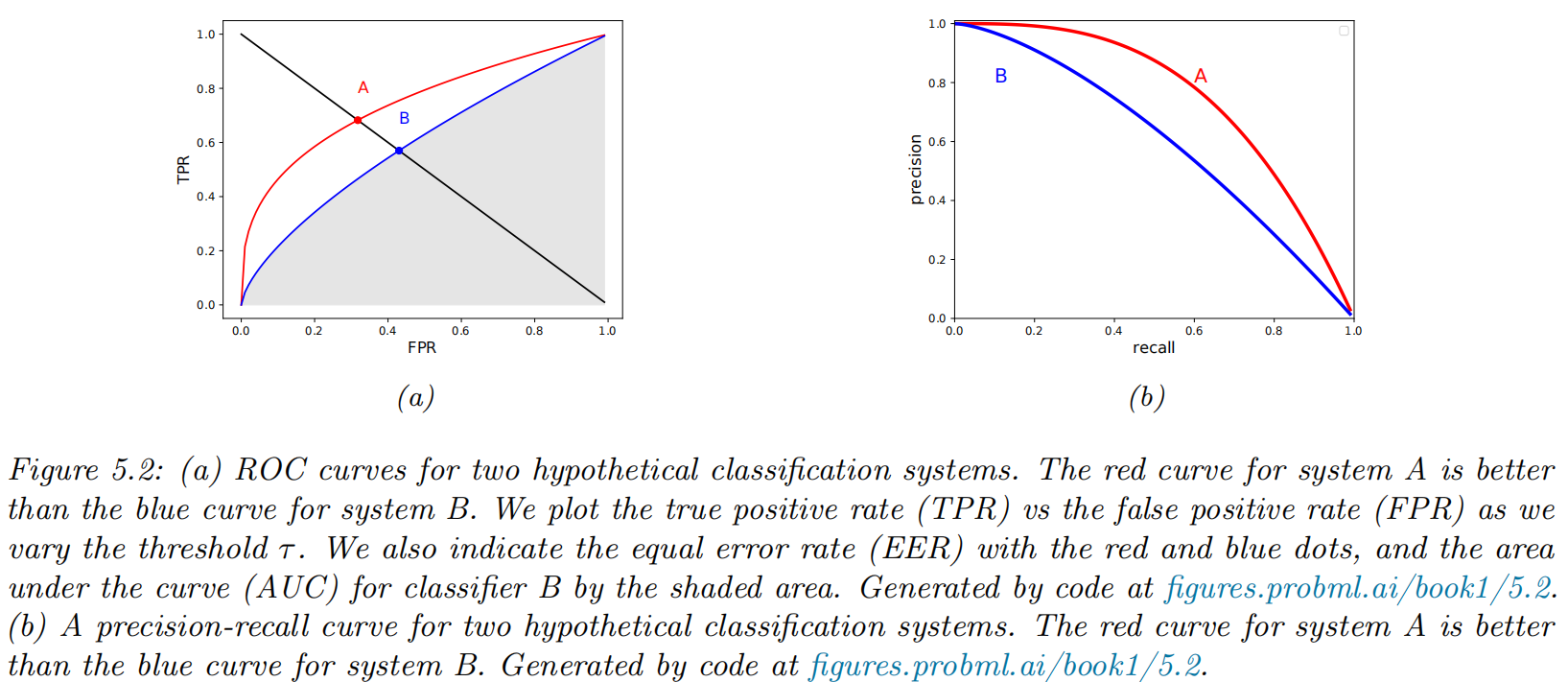
Summarizing ROC curves as a scalar

• Area Under the Curve (AUC)
  • higher AUC scores are better
  • the maximum is 1
• Equal Error Rate (EER) or cross-over rate
  • defined as the value which satisfies FPR = FNR
  • lower EER scores are better
  • the minimum is 0

Precision-recall curves

Computing precision and recall

• the precision:

$$\mathcal{P}(\tau)=p(y=1|\hat{y}=1,\tau)=\frac{TP_\tau}{TP_\tau+FP_\tau}$$

• the recall

$$\mathcal{R}(\tau)=p(\hat{y}=1|y=1,\tau)=\frac{TP_\tau}{TP_\tau+FN_\tau}$$

• If $\hat{y}_n\in\{0,1\}$ is the predicted label, and $y_n\in\{0,1\}$ is the true label, we can estimate precision and recall using

$$\mathcal{P}(\tau)=\frac{\sum_ny_n\hat{y}_n}{\sum_n\hat{y}_n}$$
$$\mathcal{R}(\tau)=\frac{\sum_ny_n\hat{y}_n}{\sum_ny_n}$$

Summarizing PR curves as a scalar

• the precision at K score: quote the precision for a fixed recall level, such as the precision of the first K = 10 entities recalled
• the interpolated precision: compute the area under the PR curve
• the average precision: the average of the interpolated precision, which is equal to the area under the interpolated PR curve
• the mean average precision or mAP: the mean of the AP over a set of different PR curves

F-scores

• Definition

$$\frac{1}{F_\beta}=\frac{1}{1+\beta^2}\frac{1}{\mathcal{P}}+\frac{\beta^2}{1+\beta^2}\frac{1}{\mathcal{R}}$$

$$F_\beta=(1+\beta^2)\frac{\mathcal{P}\cdot\mathcal{R}}{\beta^2\mathcal{P}+\mathcal{R}}=\frac{(1+\beta^2)TP}{(1+\beta^2)TP+\beta^2FN+FP}$$

• A special case: $\beta=1$

Regression problems

We assume the set of actions and states are both equal to the real
line, $\mathcal{A} = \mathcal{H} = \mathbb{R}$.

L2 loss

• the $\ell_2$ loss, also called squared error or quadratic loss

$$\ell_2(h,a)=(h-a)^2$$

• the risk function

$$R(a|\mathbf{x})=\mathbb{E}[(h-a)^2|\mathbf{x}]=\mathbb{E}[h^2|\mathbf{x}]-2a\mathbb{E}[h|\mathbf{x}]+a^2$$

• the minimum mean squared error estimate or MMSE estimate

$$\frac{\partial R}{\partial a}R(a|\mathbf{x})=-2\mathbb{E}[h|\mathbf{x}]+2a=0\Rightarrow \pi(\mathbf{x})=\mathbb{E}[h|\mathbf{x}]\int hp(h|\mathbf{x})dh$$

• The $\ell_2$ loss penalizes deviations from the truth quadratically, and thus is sensitive to outliers.

L1 loss

• the $\ell_1$ loss, also called squared error or quadratic loss

$$\ell_1(h,a)=|h-a|$$

• the optimal estimate is the posterior median

$$\Pr(h<a^*|\mathbf{x})=\Pr(h\geq a^*|\mathbf{x})=0.5$$

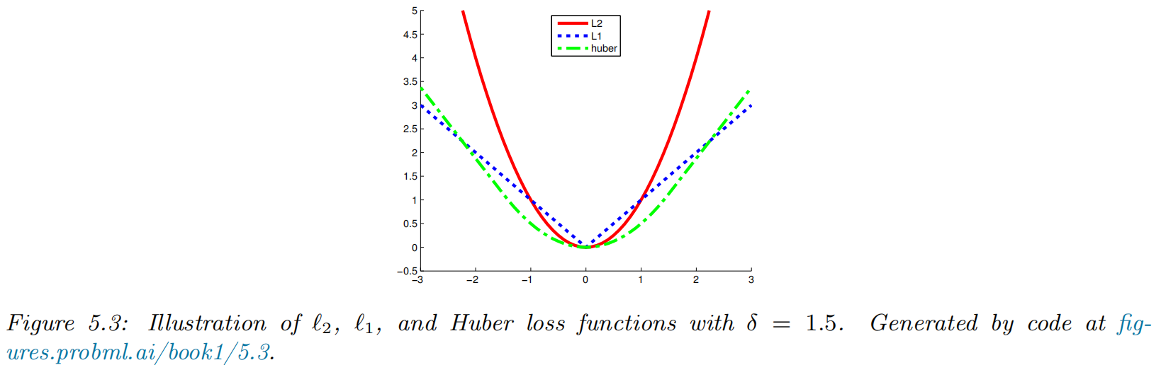
Huber loss

Let $r=h-a$,

$$l_\delta(h,a)=\left\{\begin{array}{ll}r^2/2&\text{ if }|r|\leq\delta\\\delta|r|-\delta^2/2&\text{ if }|r|>\delta\end{array}\right.$$

Probabilistic prediction problems

We assume the true “state of nature” is a distribution, $h = p(Y |x)$, the action is another distribution, $a = q(Y |x)$, and we want to pick $q$ to minimize $\mathbb{E}[l(p, q)]$ for a given $x$.

KL, cross-entropy and log-loss

A common form of loss functions for comparing two distributions is the Kullback Leibler divergence, or KL divergence, which is defined as follows:

$$D_{\mathbb{KL}(p||q)}\sum_{y\in\mathcal{Y}}p(y)\log \frac{p(y)}{q(y)}$$

• The KL is the extra number of bits we need to use to compress the data due to using the incorrect distribution $q$.

• minimize the cross-entropy

$$q^*(Y|x)=\argmin_q\mathbb{H}(q(Y|x),q(Y|x))$$

Proper scoring rules

• proper scoring rule: a loss function $f$ satisfies the follwoing

$$l(p,p)\leq l(p,q)\text{, with equality iff }p=q$$

• Brier score:

$$l(p,q)=\frac{1}{C}\sum_{c=1}^C(q(y=c|x)-p(y=c|x))^2$$

Choosing the "right" model

Bayesian hypothesis testing

• two hypothesis / model
  • null hypothesis: $M_0$
  • alternative hypothesis: $M_1$
  • 0-1 loss
  • Bayes factor: the ratio of marginal likelihoods of the two models

$$B_{1,0}=\frac{p(\mathcal{D}|M_1)}{p(\mathcal{D}|M_0)}$$

Bayes factor $BF(1,0)$	Interpretation
$BF<1/100$	Decisive evidence for $M_0$
$BF<1/10$	Strong evidence for $M_0$
$1/10<BF<1/3$	Moderate evidence for $M_0$
$1/3<BF<1$	Weak evidence for $M_0$
$1<BF<3$	Weak evidence for $M_1$
$3<BF<10$	Moderate evidence for $M_1$
$BF>10$	Strong evidence for $M_1$
$BF>100$	Decisive evidence for $M_1$

Example: Testing if a coin is fair

• test if a coin is fair
  • $H_0$: faire, i.e. $\theta=0.5$
  • $H_1$: unfair, i.e. $\theta\in[0,1]$
• marginal likelyhood under
  • $M_0$:
    $$p(\mathcal{D}|M_0)=\left(\frac{1}{2}\right)^N$$
  • $M_1$ with a Beta prior:
    $$p(\mathcal{D}|M_1)=\int p(\mathcal{D}|\theta)p(\theta)d\theta=\frac{B(\alpha_1+N_1,\alpha_0+N_0)}{B(\alpha_1,\alpha_0)}$$

Bayesian model selection

• Model Selection: pick a most apprppriate model from a set $\mathcal{M}$ of more than 2 models

$$\hat{m}=\argmax_{m\in\mathcal{M}}p(m|\mathcal{D})$$

• posterior

$$p(m|\mathcal{D})=\frac{p(\mathcal{D}|m)p(m)}{\sum_{m\in\mathcal{M}}p(\mathcal{D}|m)p(m)}$$

• uniform prior

$$p(m)=\frac{1}{|\mathcal{M}|}$$

• marginal likelyhood

$$p(\mathcal{D}|m)=\int p(\mathcal{D}|\theta,m)p(\theta|m)d\theta$$

Example: polynomial regression

Occam's razor

• Occam’s razor: the simpler the better (for the same marginal likelyhood)

• Bayesian Occam’s razor effect: the marginal likelihood will prefer the simpler model.

Connection between cross validation and marginal likelihood

Marginal likelihood is closely related to the leave-one-out cross-validation (LOO-CV) estimate.

$$p(\mathcal{D}|m)=\prod_{n=1}^Np(y_n|y_{1:n-1},x_{1:N},m)=\prod_{n=1}^Np(y_n|x_n,\mathcal{D}_{1:n-1},m)$$

where

$$p(y|x,\mathcal{D}_{1:n-1},m)=\int p(y|x,\theta)p(\theta|\mathcal{D}_{1:n-1},m)d\theta$$

Suppose we use a plugin approximation to the above distribution to get

$$p(y|x,\mathcal{D}_{1:n-1},m)\approx\int p(y|x,\theta)(\theta-\hat{\theta}_m(\mathcal{D}_{1:n-1}))d\theta=p(y|x,\hat{\theta}_m(\mathcal{D}_{1:n-1}))$$

Then we get

$$\log p(\mathcal{D}|m)\approx\sum_{n=1}^N\log p(y|x,\hat{\theta}_m(\mathcal{D}_{1:n-1}))$$

Information criteria

• the marginal likelyhood can be difficult to compute
• the result can be quite sensitive to the choice of prior

The Bayesian information criterion (BIC)

• The Bayesian information criterion or BIC can be thought of as a simple approximation to the log marginal likelihood.

$$\log p(\mathcal{D}|m)\approx\log p(\mathcal{D}|\hat{\theta}_{map})+\log p(\hat{\theta}_{map})-\frac{1}{2}|\mathbf{H}|$$

where H is the Hessian of the negative log joint $\log p(D, θ)$ evaluated at the MAP estimate $\hat{θ}_{map}$.

• Assuming uniform prior, $p(\theta)\propto1$, we can drop the prior term, and replace the MAP estimate with the MLE, $\hat{\theta}$

$$\log p(\mathcal{D}|m)\approx\log p(\mathcal{D}|\hat{\theta})-\frac{1}{2}|\mathbf{H}|$$

• the BIC score

$$J_{BIC}(m)=\log p(\mathcal{D}|\hat{\theta}_{map})-\frac{D_m}{2}\log N$$

• the BIC loss

$$\mathcal{L}_{BIC}(m)=-2\log p(\mathcal{D}|\hat{\theta}_{map})+\log N$$

Akaike information criterion

$$\mathcal{L}_{AIC}(m)=-2\log p(\mathcal{D}|\hat{\theta},m)+2D$$

• This penalizes complex models less heavily than BIC, since the regularization term is independent of $N$.
• This estimator can be derived from a frequentist perspective.

Minimum description length (MDL)

$$\mathcal{L}_{MDL}(m)=-\log p(\mathcal{D}|\hat{\theta},m)+C(m)$$

Frequentist decision theory

Computing the risk of an estimator

We define the frequentist risk of an estimator π given an unknown state of nature $\theta$ to be the expected loss when applying that estimator to data $x$ sampled from the likelihood function $p(x|\theta)$:

$$R(\theta,\pi)=\mathbb{E}_{p(x|\theta)}[l(\theta,\pi(\mathbf{x}))]$$

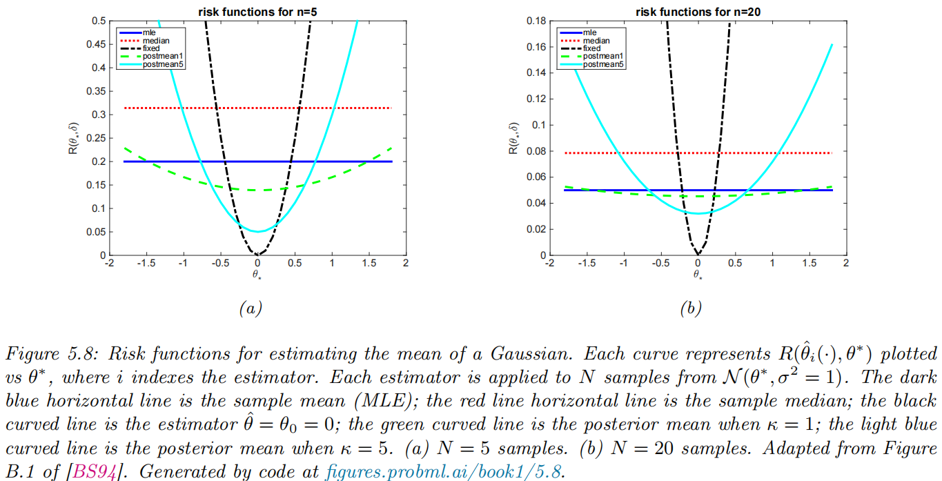
Example: estimate a Gaussian mean

• assume the data is sampled from $x_n\sim\mathcal{N}(\theta^*,\sigma^2=1)$
• quandratic loss: $\ell_2(\theta,\hat{\theta})=(\theta-\hat{\theta})^2$
• risk function: MSE
• 5 different estimators for computing $\theta$
  • sample mean: $\pi_1(\mathcal{D})=\bar{x}$
  • sample median: $\pi_2(\mathcal{D})=\text{median}(\mathcal{D})$
  • a fixed value: $\pi_2(\mathcal{D})=\theta_0$
  • $\pi_\kappa(\mathcal{D})$: the posterior mean under a $\mathcal{N}(\theta|\theta_0,\sigma^2/\kappa)$
    • weak case: $\theta_0=0,\ \kappa=1$
    • strong case: $\theta_0=0,\ \kappa=5$

$$\pi_\kappa(\mathcal{D})\frac{N}{N+\kappa}\bar{\pi}+\frac{\kappa}{N+\kappa}\theta_0=w\bar{x}+(1-w)\theta_0$$

• MSE:$MSE(\hat{\theta}|\theta^*)=\mathbb{V}[\hat{\theta}]+bias^2(\hat{\theta})$
  • sample mean:
    $$MSE(\pi_1|\theta^*)=\mathbb{V}[\bar{x}]=\frac{\sigma^2}{N}$$
  • sample median:
    $$MSE(\pi_2|\theta^*)=\frac{\pi}{2N}$$
  • fixed value:
    $$MSE(\pi_3|\theta^*)=(\theta^*-\theta_0)^2$$
  • postior:
    $$MSE(\pi_\kappa|\theta^*)=\frac{1}{(N+\kappa)^2})(N\sigma^2+\kappa^2(\theta_0-\theta^*)^2)$$

Bayes risk

• Bayes risk (integrated risk):
  $$R(\pi_0,\pi)=\mathbb{E}_{\pi_0(\theta)}[R(\theta,\pi)]=\int d\theta dx\pi_0(\theta)p(x|\theta)l(\theta,\pi(x))$$

• Bayes estimator
  $$\pi(x)=\argmin_a\int d\theta \pi_0(\theta)p(x|\theta)l(\theta,a)=\argmin_a\int d\theta p(\theta|x)l(\theta,a)$$

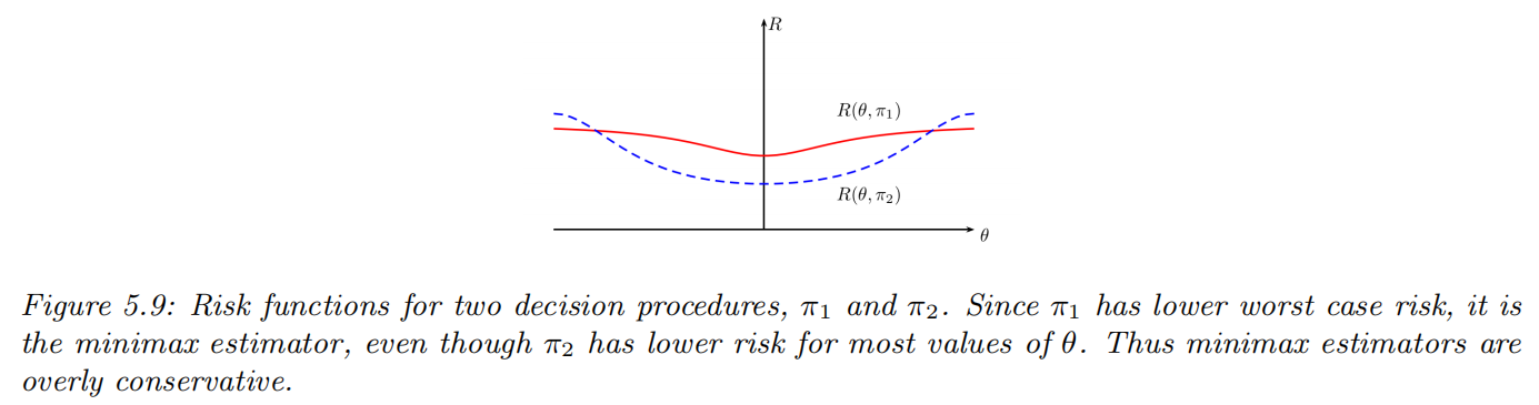
Maximum risk

• Maximum risk
  $$R_{\max}(\pi)=\sup_\theta R(\theta,\pi)$$

Empirical risk minimization

Empirical risk

• Population risk

$$R(f,p^*)=R(f)=\mathbb{E}_{p^*(x)P^*(y|x)}[l(y,f(x))]$$

• Empirical risk

  • Empirical distribution
    $$p_{\mathcal{D}}(x,y|\mathcal{D})=\frac{1}{|\mathcal{D}|}\sum_{(x_n,y_n)\in\mathcal{D}}\delta(x-x_n)\delta(y-y_n)$$
  • Empirical risk
    $$R(f,\mathcal{D})=\mathbb{E}_{p_{\mathcal{D}}(x,y)}[l(y,f(x))]=\frac{1}{N}\sum_{n=1}^Nl(y_n,f(x_n))$$

• Empirical risk minimization (ERM)
  $$\hat{f}_{ERM}=\argmin_{f\in\mathcal{H}}R(f,\mathcal{D})=\argmin_{f\in\mathcal{H}}\frac{1}{N}\sum_{n=1}^Nl(y_n,f(x_n))$$

Approximation error vs estimation error

• Notations

  • $f^{**}=\argmin_fR(f)$: function that achieves the minimal possible population risk
  • $f^*=\argmin_{f\in\mathcal{H}}R(f)$: the best function in the hypothesis space
  • $f^*_N=\argmin_{f\in\mathcal{H}}R(f,\mathcal{D})$: the prediction function that minimizes the empirical risk in the hypothesis space

• Error decomposition: approximation error ($\mathcal{E}_{app}(\mathcal{H},N)$) vs. estimation error or generalization error ($\mathcal{E}_{est}(\mathcal{H},N)$)
  $$\mathbb{E}_{p^*}[R(f^*_N)-R(f^{**})]=R(f^*)-R(f^{**})+\mathbb{E}_{p^*}[R(f^*_N)-R(f^{*})]$$

• generalization gap
  $$\mathbb{E}_{p^*}[R(f^*_N)-R(f^{*})]\approx\mathbb{E}_{p_{tr}}[l(y,f^*_N(x))]+\mathbb{E}_{p_{te}}[l(y,f^*_N(x))]$$

Regularized risk

• regularized empirical risk
  $$R_\lambda(f,\mathcal{D})=R(f,\mathcal{D})+\lambda C(f)$$
  • $C(f)$ measures the complexity of the prediction function
  • $\lambda\geq0$ is known as a hyperparameter
• parametric function form
  $$R_\lambda(\theta,\mathcal{D})=R(\theta,\mathcal{D})+\lambda C(\theta)$$
• log loss, negative log prior regularizer
  $$R_\lambda(\theta,\mathcal{D})=-\frac{1}{N}\sum_{n=1}^N\log p(y_n|x_n,\theta)-\lambda\log p(\theta)$$
  Minimizing this is equivalent to MAP estimation.

Structural risk

• how to minimize empirical risk?
  $$\hat{\lambda}=\argmin_\lambda\min_\theta R_\lambda(\theta,\mathcal{D})$$

• It does not work (optimism of the training error)
  $$\argmin_\lambda\min_\theta R_\lambda(\theta,\mathcal{D})=\argmin_\lambda\min_\theta R_\lambda(\theta,\mathcal{D})+\lambda C(\theta)$$

• structural risk minimization: If we knew the regularized population risk $R_\lambda(\theta)$, instead of the regularized empirical risk $R_\lambda(\theta,\mathcal{D})$, we could use it to pick a model of the right complexity (e.g., value of $\lambda$)

• two methods to estimate the population risk for a given model (value of $\lambda$)

  • cross-validation
  • statistical learning theory

Cross-validation

• partition the dataset into two
  • training set $\mathcal{D}_\text{train}$: to fit/train the model
  • validation set $\mathcal{D}_\text{valid}$ or holdout set: to assess the risk
• the empirical risk on the dataset
  $$R_\lambda(\theta,\mathcal{D})=\frac{1}{|\mathcal{D}|}\sum_{(x,y)\in\mathcal{D}}l(y,f(x;\theta))+\lambda C(\theta)$$
• $\hat{\theta}_\lambda=\argmin_\theta R_\lambda(\theta,\mathcal{D})$
• validation risk: use the unregularized empirical risk on the validation set as an estimate of the population risk
  $$R^{val}_\lambda=R_0(\hat{\theta}_\lambda(\mathcal{D}_\text{train}),\mathcal{D}_\text{valid})$$
• K-folds cross validation (CV):
  • split the training data into K folds
  • for each fold $k\in\{1,\dots,K\}$, we train on all the folds but the k’th
  • test on the k’th
• cross-validated risk
  $$R^\text{CV}_\lambda=\frac{1}{K}\sum_{k=1}^KR_0(\hat{\theta}_\lambda(\mathcal{D}_{-k}),\mathcal{D}_{k})$$
• optimal parameters
  • optimal hyperparameters: $\hat{\lambda}=\argmin_\lambda R_\lambda^\text{CV}$
  • optimal model parameters: $\hat{\theta}=\argmin_\theta R_{\hat{\lambda}}(\theta,\mathcal D)$

Information Theory

Entropy

The entropy of a probability distribution can be interpreted as a measure of uncertainty, or lack of predictability, associated with a random variable drawn from a given distribution. We can also use entropy to define the information content of a data source.

Entropy of $p$	Hard/Easy to predict $X_n$	Information content of $\mathcal{D}$
high	hard	high
low	easy	low

Entropy for discrete random variables

The entropy of a discrete random variable $X$ with distribution $p$ over $K$ states is defined by

$$\mathbb{H}(X)=-\sum^K_{k=1}p(X=k)\log_2p(X=k)=-\mathbb{E}_X[\log p(X)]$$

• When we use log base 2, the units are called bits (short for binary digits).
• When we use log base $e$, the units are called nats.

Cross entropy

The cross entropy between distribution $p$ and $q$ is defined by

$$\mathbb{H}(p,q)=-\sum^K_{k=1}p_k\log q_k$$

The cross entropy is the expected number of bits needed to compress some data samples drawn from distribution $p$ using a code based on distribution $q$. This can be minimized by setting $q = p$, in which case the expected number of bits of the optimal code is $\mathbb{H}(p, p) = \mathbb{H}(p)$ — this is known as Shannon’s source coding theorem.

Joint entropy

The joint entropy of two random variables $X$ and $Y$ is defined as

$$\mathbb{H}(X,Y)=-\sum_{x,y}p(x,y))\log_2 p(x,y)$$

For example, consider choosing an integer from 1 to 8, $n\in\{1, . . . , 8\}$. Let $X(n) = 1$ if $n$ is even, and $Y (n) = 1$ if $n$ is prime:

$n$	1	2	3	4	5	6	7	8
$X$	0	1	0	1	0	1	0	1
$Y$	0	1	1	0	1	0	1	0

The joint distribution is

$p(X,Y)$	$Y=0$	$Y=1$
$X=0$	$1/8$	$3/8$
$Y=1$	$3/8$	$1/8$

so the joint entropy is given by

$$\mathbb{H}(X,Y)=-\left[\frac{1}{8}\log_2\frac{1}{8}+\frac{3}{8}\log_2\frac{3}{8}+\frac{3}{8}\log_2\frac{3}{8}+\frac{1}{8}\log_2\frac{1}{8}\right]=1.81\ bits$$

Consider the marginal entropys:

$$\mathbb{H}(X)=\mathbb{H}(Y)=-\left[\frac{1}{2}\log_2\frac{1}{2}+\frac{1}{2}\log_2\frac{1}{2}\right]=1$$

We observe that

$$1.81=\mathbb{H}(X,Y)<\mathbb{H}(X)+\mathbb{H}(Y)=2$$

In general, the above inequality is always valid. If X and Y are independent, then $\mathbb{H} (X, Y ) = \mathbb{H }(X) + \mathbb{H} (Y )$, so the bound is tight. This makes intuitive sense: when the parts are correlated in some way, it reduces the “degrees of freedom” of the system, and hence reduces the
overall entropy.

Another observation is that

$$\mathbb{H}(X,Y)\geq\max\left\{\mathbb{H}(X)+\mathbb{H}(Y)\right\}$$

this says combining variables together does not make the entropy go down: you cannot reduce uncertainty merely by adding more unknowns to the problem, you need to observe some data.

Conditional entropy

The conditional entropy of $Y$ given $X$ is the uncertainty we have in $Y$ after seeing $X$, averaged over possible values for $X$:

$$\mathbb{H}(Y|X)=\mathbb{E}_{p(X)}\left[\mathbb{E}\left(p\left(Y|X\right)\right)\right]=\mathbb{H}(X,Y)-\mathbb{H}(X)$$

It is straight forward to verify that:

• $\mathbb{H}(Y|X)=\mathbb{H}(X,Y)-\mathbb{H}(X)\leq\mathbb{H}(X)+\mathbb{H}(Y)-\mathbb{H}(X)=\mathbb{H}(Y)$
• $\mathbb{H}(X_1,X_2,\dots,X_n)=\sum_{i=1}^n\mathbb{H}(X_i|X_1,\dots,X_{i-1})$

Perplexity

The perplexity of a discrete probability distribution $p$ is defined as

$$\text{perplexity}(p)=2^{\mathbb{H}(p)}$$

It is often interpreted as a measure of predictability. Suppose we have an empirical distribution based on data $\mathcal{D}$:

$$p_{\mathcal{D}}(x|\mathcal{D})=\frac{1}{N}\sum_{n=1}^N\delta_{x_n}(x)$$

We can measure how well $p$ predicts $\mathcal{D}$ by computing

$$\text{perplexity}(p_{\mathcal{D}},p)=2^{\mathbb{H}(p_{\mathcal{D}},p)}$$

Differential entropy for continuous random variables *

If $X$ is a continuous random variable with pdf $p(x)$, we define the differential entropy as

$$h(X)=-\int_{\mathcal{X}}dxp(x)\log p(x)$$

Differential entropy can be negative since pdf’s can be bigger than 1.

Example: Entropy of a Gaussian

The entropy of a d-dimensional Gaussian is

$$h(\mathcal{N}(\mathbf{\mu},\mathbf{\Sigma}))=\frac{1}{2}\ln |2\pi e\mathbf{\Sigma}|=\frac{1}{2}\ln[(2\pi e)^d|\mathbf{\Sigma}|]=\frac{d}{2}+\frac{d}{2}\ln(2\pi)+\frac{1}{2}\ln|\mathbf{\Sigma}|$$

In the 1d case, this becomes

$$h(\mathcal{N}(\mu,\sigma^2))=\frac{1}{2}\ln[2\pi e\sigma^2]$$

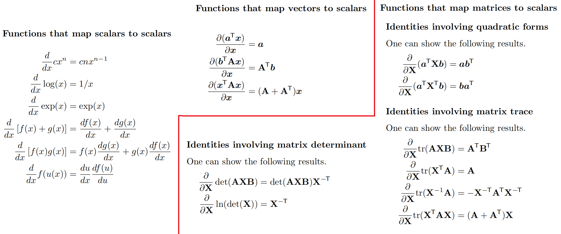
Linear Algebra

Matrix calculus

Derivatives

$$f'(x)=\lim_{h\rightarrow0}\frac{f(x+h)-f(x)}{h}$$

Gradients

• Patial derivative:
  $$\frac{\partial f}{\partial x_i}=\lim_{h\rightarrow0}\frac{f(\mathbf{x}+h\mathbf{e}_i)-f(\mathbf{x})}{h}$$
• Gradient:
  $$\mathbf{g}=\frac{\partial f}{\partial \mathbf{x}}=\nabla f=\left(\begin{array}{c}\frac{\partial f}{\partial x_1}\\\frac{\partial f}{\partial x_2}\\\vdots\frac{\partial f}{\partial x_n}\end{array}\right)$$
• Gradient evaluated at point $\mathbf{x}^*$:
  $$\mathbf{g}(\mathbf{x}^*)=\left.\frac{\partial f}{\partial \mathbf{x}}\right|_{\mathbf{x}^*}$$

Directional derivative

The directional derivative measures how much the function $f:\mathbb{R}^n\rightarrow\mathbb{R}$ changes along a direction $\mathbf{v}$ in space. It is defined as follows

$$\mathcal{D}_{\mathbf{v}}f(\mathbf{x})=\lim_{h\rightarrow0}\frac{f(\mathbf{x}+h\mathbf{v})-f(\mathbf{x})}{h}$$

Note that the directional derivative along $\mathbf{v}$ is the scalar product of the gradient g and the vector $\mathbf{v}$:

$$\mathcal{D}_{\mathbf{v}}f(\mathbf{x})=\nabla f(\mathbf{x})\cdot\mathbf{v}$$

Total derivative

Suppose that some of the arguments to the function depend on each other. Concretely, suppose the function has the form $f(t, x(t), y(t))$. We define the total derivative of $f$ wrt t as follows:

$$\dfrac{df}{dt}=\dfrac{\partial f}{\partial t}+\dfrac{\partial f}{\partial x}\dfrac{d x}{d t}+\dfrac{\partial f}{\partial y}\dfrac{d y}{d t}$$

If we multiply both sides by the differential $dt$, we get the total differential

$$df=\dfrac{\partial f}{\partial t}dt+\dfrac{\partial f}{\partial x}dx+\dfrac{\partial f}{\partial y}dy$$

This measures how much f changes when we change $t$, both via the direct effect of $t$ on $f$, but also indirectly, via the effects of t on $x$ and $y$.

Jacobian

Consider a function that maps a vector to another vector, $\mathbf{f}:\mathbb{R}^n\rightarrow\mathbb{R}^m$. The Jacobian matrix of this function is an $m \times n$ matrix of partial derivatives:

$$\mathbf{J_f}(\mathbf{x})=\dfrac{\partial \mathbf{f}}{\partial \mathbf{x}^T}=\left(\begin{array}{ccc}\frac{\partial f_1}{\partial x_1} & \cdots & \frac{\partial f_1}{\partial x_n}\\\vdots&\ddots&\vdots\\\frac{\partial f_m}{\partial x_1} & \cdots &\frac{\partial f_m}{\partial x_n}\end{array}\right)=\left(\begin{array}{c}\nabla f_1(\mathbf{x})^T\\\vdots\\\nabla f_m(\mathbf{x})^T\end{array}\right)$$

Multiplying Jacobians and vectors

The Jacobian vector product or JVP is defined to be the operation that corresponds to right multiplying the Jacobian matrix $\mathbf{J}\in\mathbb{R}^{m\times n}$ by a vector $\mathbf{v}\in\mathbb{R}^{n}$:

$$\mathbf{J_f}(\mathbf{x})\mathbf{v}=\left(\begin{array}{c}\nabla f_1(\mathbf{x})^T\\\vdots\\\nabla f_m(\mathbf{x})^T\end{array}\right)\mathbf{v}=\left(\begin{array}{c}\nabla f_1(\mathbf{x})^T\mathbf{v}\\\vdots\\\nabla f_m(\mathbf{x})^T\mathbf{v}\end{array}\right)$$

So we can see that we can approximate this numerically using just 2 calls to $\mathbf{f}$.

The vector Jacobian product or *VJP is defined to be the operation that corresponds to left-multiplying the Jacobian matrix $\mathbf{J}\in\mathbb{R}^{m\times n}$ by a vector $\mathbf{u}\in\mathbb{R}^{m}$:

$$\mathbf{u}^T\mathbf{J_f}(\mathbf{x})=\mathbf{u}^T\left(\frac{\partial \mathbf{f}}{\partial x_1},\cdots,\frac{\partial \mathbf{f}}{\partial x_n}\right)=\left(\mathbf{u}\cdot\frac{\partial \mathbf{f}}{\partial x_1},\cdots,\mathbf{u}\cdot\frac{\partial \mathbf{f}}{\partial x_n}\right)$$

Jacobian of a composition

Let $h(\mathbf{x}) = g(f(\mathbf{x}))$. By the chain rule of calculus, we have

$$\mathbf{J_h}(\mathbf{x})=\mathbf{J_g}(f(\mathbf{x}))\mathbf{J_f}(\mathbf{x})$$

Hessian

For a function f : Rn → R that is twice differentiable, we define the Hessian matrix as the (symmetric) $n \times n$ matrix of second partial derivatives:

$$\mathbf{H_f}(\mathbf{x})=\dfrac{\partial^2 f}{\partial \mathbf{x}^2}=\nabla^2f=\left(\begin{array}{ccc}\frac{\partial^2 f}{\partial x_1^2} & \cdots & \frac{\partial^2 f}{\partial x_1\partial x_n}\\\vdots&\ddots&\vdots\\\frac{\partial^2 f}{\partial x_n\partial x_1} & \cdots &\frac{\partial^2 f}{\partial x_n^2}\end{array}\right)$$

The Hessian is the Jacobian of the gradient.

Gradients of commonly used functions