Machine Learning in Finance
L01 Introduction to Financial Machine Learning
Finance and ...
关于金融与金融工程
“金融”的意义
-
黄洪:
- 金融一词并非古已有之 。‘金’与‘融’这两个字,是极古老的中国字,可是这两个字连在一起组成一个既不能单独用‘金’字解释也不能单独用‘融’字解释的词—金融—则不见于任何古籍。《康熙字典》及其以前的所有辞书均无金与融连用的记栽。作为一个词条,最早见于1915年初版的《辞源》和1937年初版的《辞海》。这说明,至迟在19世纪下半叶,金与融这两个字组成的词已经定型并在经济领域中相当广泛地使用;两部辞书的释义均指通过信用中介机构的货币资金融通。”
- 连起来的‘金融’始于何时,无确切考证,最大可能是来自明治维新的日本。那一阶段,有许多西方经济学的概念就是从日本引进的—直接把日语翻译西文的汉字搬到中国来
-
艾俊川:古籍中“金融”义指“黄金融制而成” 。
-
张辑颜:金融者,金币之融通状况之谓也。故金融学科,为研究金币之融通状况,及其与国家财政,民生经济,所生各种关系之学科也。金融之名词译自日本:盖日本以金币为本位,故称金融。”
-
艾俊川:
- (日本)“金融”二字连用之词,显然是“金钱融通”的缩略 (1875)
- 将“金融”译为英文 The Circulation of Money (1897,1911)
- 在此后十年间,日本书籍报刊中“金融”一词爆发性使用,词义也开始转变,被用来指称与货币和信用有关的交易与经济活动,日译本“金融”对应英语名词“money market"(1883)
-
孙大权:
- 1902年4月22日,梁启超独自编辑的《新民丛报》登载了关于“金融”一词的“问答”。东京爱读生问: “日本书中金融二字其意云何? 中国当以何译之?”梁启超答道: “金融者指金银行情之变动涨落。……日本言金融,取金钱融通之意,如吾古者以泉名币也。沿用之似亦可乎。
- Finance最初在中国和日本均为与“财政”有关的含义。1929年3月,萧纯锦在编译自美国的《经济学》里指出: “‘金融’(在英文为Finance)”
- 1941 年,由何廉、陈岱孙、陈启修等32位著名经济学家审查通过,由国民政府教育部公布的《经济学名词》中,Finance对译为“财政,金融”; Money Market对译为“金融市场”; Money对译为“货币”; Currency对译为“通货”。“金融”唯一的对应译词为Finance,这样,金融与Finance对译就成为民国主流经济学家认可的用法。
- 1902年4月22日,梁启超独自编辑的《新民丛报》登载了关于“金融“一词的“问答”。东京爱读生问: “日本书中金融二字其意云何? 中国当以何译之?”梁启超答道: “金融者指金银行情之变动涨落。……日本言金融,取金钱融通之意,如吾古者以泉名币也。沿用之似亦可乎。
- Finance最初在中国和日本均为与“财政”有关的含义。1929年3月,萧纯锦在编译自美国的《经济学》里指出: “‘金融’(在英文为Finance) ”
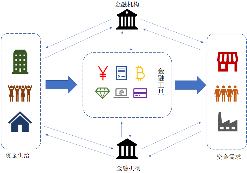
金融活动
金融研究
- 期刊
| 期刊 | 创刊年份 |
|---|---|
| The Journal of Finance | 1946 |
| Journal of Financial and Quantitative Analysis | 1966 |
| Journal of Financial Economics | 1974 |
| 金融研究 | 1980 |
| The Review of Financial Studies | 1988 |
- 学会/协会
| 协会 | 创办年份 |
|---|---|
| The American Finance Association | 1939 |
| 中国金融学会 | 1950 |
| Western Finance Association | 1965 |
| European Finance Association | 1974 |
| Society for Financial Studies | 1987 |
什么是金融?
-
金融学研究资源如何有效地在不确定的条件下跨期分配
-
金融学研究的几个重要问题:
- 资产定价
- 风险管理
- 资产配置
与金融相关的诺贝尔经济学奖
-
1981: James Tobin “for his analysis of financial markets and their relations to expenditure decisions, employment, production and prices”.
-
1985: Franco Modigliani “for his pioneering analyses of saving and of financial markets”.
-
1990: Harry M. Markowitz, Merton H. Miller and William F. Sharpe “for their pioneering work in the theory of financial economics”.
-
1997: Robert C. Merton and Myron S. Scholes “for a new method to determine the value of derivatives”.
-
2003: Robert F. Engle III “for methods of analyzing economic time series with time-varying volatility (ARCH)”. Clive W.J. Granger “for methods of analyzing economic time series with common trends (cointegration)”
-
2013: Eugene F. Fama, Lars Peter Hansen and Robert J. Shiller “for their empirical analysis of asset prices”.
-
2017: Richard H. Thaler “for his contributions to behavioural economics”.
什么是金融工程?
什么是工程?

-
工程是...
- 利用基本的材料、工具、部件、器材、结构
- 在相关基础理论的指导下、按照某(些)种工艺、技术进行组合、装配
- 实现一定的功能、满足特定需求、解决具体问题
兹维博迪的定义
Financial engineering is the application of science-based mathematical models to decisions about saving, investing, borrowing, lending, and managing risk. -- by Zvi Bodie
- 金融工程是金融理论与工程方法的结合
- 金融工程不是一个工程学科
- 金融工程的发展基于现代金融理论
- 金融工程是一个应用学科
国际数量金融协会(iaqf)对金融工程的介绍
-
Financial engineering is the application of mathematical methods to the solution of problems in finance. It is also known as financial mathematics, mathematical finance, and computational finance.
-
Financial engineering draws on tools from applied mathematics, computer science, statistics, and economic theory.
-
Investment banks, commercial banks, hedge funds, insurance companies, corporate treasuries, and regulatory agencies employ financial engineers.
-
These businesses apply the methods of financial engineering to such problems as new product development, derivative securities valuation, portfolio structuring, risk management, and scenario simulation.
-
Quantitative analysis has brought innovation, efficiency and rigor to financial markets and to the investment process.
-
As the pace of financial innovation accelerates, the need for highly qualified people with specific training in financial engineering continues to grow in all market environments.
金融工程的研究领域

金融工程的核心问题
-
核心问题
- 资产定价(基础资产、衍生工具、复杂的结构化产品)
- 组合管理/优化
- 风险管理
-
原理与方法
- 合成与复制
- 无套利动态过程
- 风险中性
合成与复制
-
BofA Finds Way to Gain From Alibaba IPO Even After Advisory Snub
- 思路:做多阿里巴巴的主要股东(Softbank、Yahoo),同时做空非阿里巴巴收入的成分
- BAML的做法:买Soft bank,卖Sprint,卖Yahoo Japan,卖KDDI
-
期权定价:用含有期权的组合复制无风险证券
- 做空一份期权合约
- 做多若干股股票
无套利动态过程
-
套利机会存在的条件
- 存在两个不同的资产组合,它们的未来现金流相同,但它们的成本却不同
- 存在两个成本相同的组合,第一个组合在所有可能状态下的现金流都不低于第二个组合,而且至少存在一种状态,在此状态下第一个组合的现金流大于第二个组合
- 一个组合的成本为零,但在所有可能状态下,这个组合的损益都不小于零,而且至少存在一种状态,在此状态下这个组合的损益要大于零
-
套利的实现
- 买入被低估的资产(组合),卖出被高估的资产(组合)
- 通过融资/融券使初始投资为零
- 在期末获得正的利润
-
无套利动态过程
风险中性
-
风险中性定价理论有两个最基本的假设:
- 在一个投资者都是风险中性的世界里,所有证券的预期收益率均为无风险收益率
- 投资者的投资成果体现为用无风险利率贴现收益现金流得到的现值
-
无风险的套利机会出现时
- 市场参与者的套利活动与其对风险的态度无关(套利分析时未用到风险偏好信息)
- 无套利均衡分析的过程和结果与市场参与者的风险偏好无关
- 因此,假设风险中性世界(风险中性定价)简化分析
-
从风险中性世界进入到风险厌恶或者风险喜好的世界时:
- (概率分布发生变化)资产的预期收益率发生变化
- 资产任何损益(或现金流)所适用的贴现率发生改变
- 以上两个变化效果互相抵消
金融工程发展的历史逻辑
-
历史背景
- 经济全球化与金融自由化
-
理论基础
- 现代投资组合理论:Markowitz (1952)
- 资本资产定价模型:Sharpe (1964),Lintner (1964),Treynor (1964)
- 期权定价理论:Black and Scholes (1973)
-
技术条件
- 信息技术与计算能力的发展(计算机、互联网、并行计算、云计算)
- 最优化理论与算法的进展
- 大数据、人工智能
-
数理基础
- 概率论与随机过程的严格化
- 宇航科学与随机控制
关于金融工程教育
-
金融工程的学历教育项目
- 几乎没有金融工程的本科项目
- 有许多(授课式/专业型)硕士研究生项目 (Financial Engineering, Quantitative Finance, Mathematical Finance, Financial Mathematics)
- 有一些博士项目专注该领域
- 学位由工程学院、数学系、统计系、运筹与管理科学系等院系授予
- Ranking & Placement: Quantnet Ranking, Program Websites, LinkedIn
-
课程与技能
- 经济学与金融学
- 数学、理论物理
- 运筹学与统计学
- 信息理论、编程
-
金融工程师的专业背景
- 火箭科学家、应用数学家、运筹学、计算机科学家
- 金融工程项目的毕业生
Research Methods
Quantitative Methods in Finance
1827 Brown
The Scottish botanist, Robert Brown, gave his name to the random motion of small particles in a liquid. This idea of the random walk has permeated many scientific fields and is commonly used as the model mechanism behind a variety of unpredictable continuous-time processes. The lognormal random walk based on Brownian motion is the classical paradigm for the stock market. See Brown (1827).
1900 Bachelier
the concept of Brownian motion.} He developed a mathematical theory for random walks, a theory rediscovered later by Einstein. He proposed a model for equity prices, a simple normal distribution, and built on it a model for pricing the almost unheard of options. His model contained many of the seeds for later work, but lay `dormant' for many, many years. It is told that his thesis was not a great success and, naturally, Bachelier's work was not appreciated in his lifetime. See Bachelier (1995).
1911 Richardson
Most option models result in diffusion-type equations. And often these have to be solved numerically. The two main ways of doing this are Monte Carlo and finite differences (a sophisticated version of the binomial model). The very first use of the finite difference method, in which a differential equation is discretized into a difference equation, was by Lewis Fry Richardson in 1911, and used to solve the diffusion equation associated with weather forecasting. See Richardson (1922). Richardson later worked on the mathematics for the causes of war.
1923 Wiener
Norbert Wiener developed a rigorous theory for Brownian motion, the mathematics of which was to become a necessary modelling device for quantitative finance decades later. The starting point for almost all financial models, the first equation written down in most technical papers, includes the Wiener process as the representation for randomness in asset prices. See Wiener (1923).
1950s Samuelson
The 1970 Nobel Laureate in Economics, Paul Samuelson, was responsible for setting the tone for subsequent generations of economists. Samuelson 'mathematized' both macro and micro economics. He rediscovered Bachelier's thesis and laid the foundations for later option pricing theories. His approach to derivative pricing was via expectations, real as opposed to the much later risk-neutral ones. See Samuelson (1995)
1951 It
Where would we be without stochastic or It calculus? (Some people even think finance is only about It calculus.) Kiyosi It showed the relationship between a stochastic differential equation for some independent variable and the stochastic differential equation for a function of that variable. One of the starting points for classical derivatives theory is the lognormal stochastic differential equation for the evolution of an asset. It's lemma tells us the stochastic differential equation for the value of an option on that asset.
In mathematical terms, if we have a Wiener process with increments that are normally distributed with mean zero and variance dt then the increment of a function is given by
This is a very loose definition of It's lemma but will suffice. See It (1951).
1952 Markowitz
Harry Markowitz was the first to propose a modern quantitative methodology for portfolio selection. This required knowledge of assets' volatilities and the correlation between assets. The idea was extremely elegant, resulting in novel ideas such as 'efficiency' and 'market portfolios'. In this Modern Portfolio Theory, Markowitz showed that combinations of assets could have better properties than any individual assets. What did 'better' mean? Markowitz quantified a portfolio's possible future performance in terms of its expected return and its standard deviation. The latter was to be interpreted as its risk. He showed how to optimize a portfolio to give the maximum expected return for a given level of risk. Such a portfolio was said to be `efficient'. The work later won Markowitz a Nobel Prize for Economics but is rarely used in practice because of the difficulty in measuring the parameters volatility, and especially correlation, and their instability.
1963 Sharpe, Lintner and Mossin
William Sharpe of Stanford, John Lintner of Harvard and Norwegian economist Jan Mossin independently developed a simple model for pricing risky assets. This Capital Asset Pricing Model (CAPM) also reduced the number of parameters needed for portfolio selection from those needed by Markowitz's Modern Portfolio Theory,
1966 Fama
Eugene Fama concluded that stock prices were unpredictable and coined the phrase 'market efficiency'. Although there are various forms of market efficiency, in a nutshell the idea is that stock market prices reflect all publicly available information, that no person can gain an edge over another by fair means. See Fama (1966).
1960s Sobol, Faure, Hammersley, Haselgrove, Halton . . .
Many people were associated with the definition and development of quasi random number theory or low-discrepancy sequence theory. The subject concerns the distribution of points in an arbitrary number of dimensions so as to cover the space as efficiently as possible, with as few points as possible. The methodology is used in the evaluation of multiple integrals among other things. These ideas would find a use in finance almost three decades later. See Sobol (1967), Faure (1969), Hammersley and Handscomb (1964), Haselgrove (1961) and Halton (1960).
1968 Thorp
Ed Thorp's first claim to fame was that he figured out how to win at casino Blackjack, ideas that were put into practice by Thorp himself and written about in his best-selling Beat the Dealer, the 'book that made Las Vegas change its rules'. His second claim to fame is that he invented and built, with Claude Shannon, the information theorist, the world's first wearable computer. His third claim to fame is that he was the first to use the 'correct' formula for pricing options, formula that were rediscovered and originally published several years later by the next three people on our list. Thorp used these formula to make a fortune for himself and his clients in the first ever quantitative finance-based hedge fund. See Thorp (2002) for the story behind the discovery of the Black-Scholes formula.
1973 Black, Scholes and Merton
Fischer Black, Myron Scholes and Robert Merton derived the Black-Scholes equation for options in the early seventies, publishing it in two separate papers in 1973 (Black & Scholes, 1973, and Merton, 1973). The date corresponded almost exactly with the trading of call options on the Chicago Board Options Exchange. Scholes and Merton won the Nobel Prize for Economics in 1997. Black had died in 1995.
1974 Merton, again
In 1974 Robert Merton (Merton, 1974) introduced the idea of modelling the value of a company as a call option on its assets, with the company's debt being related to the strike price and the maturity of the debt being the option's expiration. Thus was born the structural approach to modelling risk of default, for if the option expired out of the money (i.e. assets had less value than the debt at maturity) then the firm would have to go bankrupt.
Credit risk became big, huge, in the 1990s. Theory and practice progressed at rapid speed during this period, urged on by some significant credit-led events, such as the Long Term Capital Management mess. One of the principals of LTCM was Merton who had worked on credit risk two decades earlier. Now the subject really took off, not just along the lines proposed by Merton but also using the Poisson process as the model for the random arrival of an event, such as bankruptcy or default. For a list of key research in this area see Schönbucher (2003).
1977 Boyle
Phelim Boyle related the pricing of options to the simulation of random asset paths. He showed how to find the fair value of an option by generating lots of possible future paths for an asset and then looking at the average that the option had paid off. The future important role of Monte Carlo simulations in finance was assured. See Boyle (1977).
1977 Vasicek
So far quantitative finance hadn't had much to say about pricing interest rate products. Some people were using equity option formula for pricing interest rate options, but a consistent framework for interest rates had not been developed. This was addressed by Vasicek. He started by modelling a short-term interest rate as a random walk and concluded that interest rate derivatives could be valued using equations similar to the Black-Scholes partial differential equation.
1979–81 Harrison, Kreps, Pliska
1979-81 Harrison, Kreps, Pliska Until these three came onto the scene quantitative finance was the domain of either economists or applied mathematicians. Mike Harrison and David Kreps, in 1979, showed the relationship between option prices and advanced probability theory, originally in discrete time. Harrison and Stan Pliska in 1981 used the same ideas but in continuous time. From that moment until the mid 1990s applied mathematicians hardly got a look in. Theorem, proof everywhere you looked. See Harrison and Kreps (1979) and Harrison and Pliska (1981).
1986 Ho and Lee
One of the problems with the Vasicek framework for interest rate derivative products was that
it didn't give very good prices for bonds, the simplest of fixed income products. If the model couldn't even get bond prices right, how could it hope to correctly value bond options? Thomas Ho and Sang-Bin Lee found a way around this, introducing the idea of yield curve fitting or calibration. See Ho and Lee (1986).
1992 Heath, Jarrow and Morton
Although Ho and Lee showed how to match theoretical and market prices for simple bonds, the methodology was rather cumbersome and not easily generalized. David Heath, Robert Jarrow and Andrew Morton took a different approach. Instead of modelling just a short rate and deducing the whole yield curve, they modelled the random evolution of the whole yield curve. The initial yield curve, and hence the value of simple interest rate instruments, was an input
to the model. The model cannot easily be expressed in differential equation terms and so relies on either Monte Carlo simulation or tree building. The work was well known via a working paper, but was finally published, and therefore made respectable in Heath, Jarrow and Morton (1992).
Finance & Fintech
Fintech
Financial Stability Board (FSB) "Monitoring of FinTech"
The FSB understands FinTech as technologically enabled innovation in financial services that could result in new business models, applications, processes or products with an associated material effect on financial markets and institutions and the provision of financial services.
中国人民银行《金融科技(FinTech)发展规划(2019-2021年)》
金融科技是技术驱动的金融创新(该定义由金融稳定理事会(FSB)于2016年提出,目前已成为全球共识),旨在运用现代科技成果改造或创新金融产品、经营模式、业务流程等,推动金融发展提质增效。
Investopedia
Financial technology (Fintech) is used to describe new tech that seeks to improve and automate the delivery and use of financial services.
CFA ® Program Curriculum
In its broadest sense, the term “fintech” generally refers to technology-driven innovation occurring in the financial services industry. For the purposes of this reading, fintech refers to technological innovation in the design and delivery of financial services and products.
CCB
Fintech=A(rtificial Intelligence)+B(igData)+C(loud Computing)+D(LT)+M(obile Internet)+I(oT)+X
Fintech应用领域:CFA ® Program Curriculum
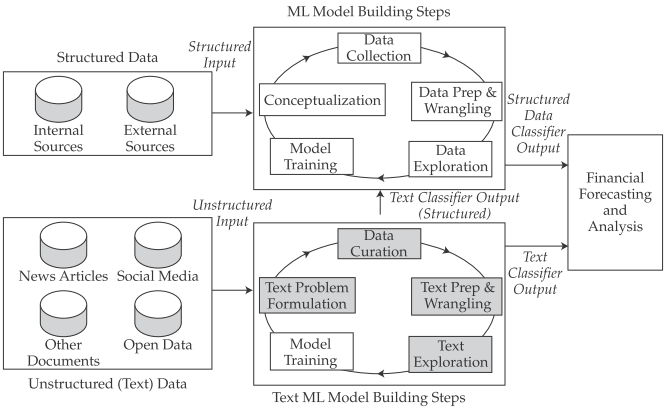
- Analysis of large datasets.
- Analytical tools. For extremely large datasets, techniques involving artificial intelligence (AI)。
- Automated trading.
- Automated advice (Robo-advisers)
- Financial record keeping (DLT)
Big Data & Data Science
Big Data (4v)
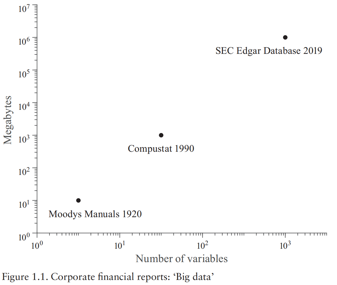
- Volume: The amount of data collected in files, records, and tables is very large, representing many millions, or even billions, of data points (GB->TB->PB->EB->ZB).
- Velocity: The speed with which the data are communicated is extremely great. Real- time or near- real- time data have become the norm in many areas.
- Variety: The data are collected from many different sources and in a variety of formats, including structured data (e.g., SQL tables or CSV files), semi-structured data (e.g., HTML code), and unstructured data (e.g., video messages).
- Value: Low value density.
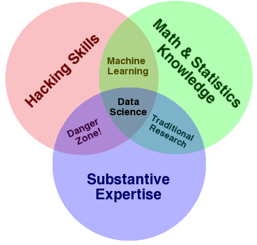
Data Science
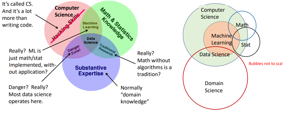
- The Conway Venn diagram for data science
Financial Forcasting with Big Data
