专题： 金融工程与风险管理

---

• 专题： 金融工程与风险管理
  • Financial Risk Management Fundamental
    • Financial Risk
      • Definition
      • Contributory factors: volatile environment
      • Contributory factors: growth in trading activity
      • Contributory factors: advances in IT
    • Financial Risk Management before VaR
      • Risk measurement before VaR
      • Gap Analysis
      • PV01 Analysis
      • Duration Analysis
      • Convexity
      • Pros and cons of duration-convexity
      • Scenario Analysis
      • Portfolio Theory
      • Derivatives risk measures
    • Value at Risk (VaR)
      • Value at Risk
      • RiskMetrics
      • Portfolio theory and VaR
      • Attractions of VaR
      • Uses of VaR
      • Criticisms of VaR
  • Advanced Risk Models: Univariate
    • Value-at-Risk (VaR)
      • VaR Parameters: The Confidence Level (cl)
      • VaR Parameters: The Holding Period (hp)
      • VaR Surface
      • Determine the Confidence Level
      • Determine the Holding Period
      • Limitation of VaR
      • VaR uninformative of tail losses
      • VaR creates perverse incentives
      • VaR can discourage diversification
      • VaR not subadditive
    • Coherent Measure of Risk
      • Coherent Risk Measures
      • Implications of coherence
      • Alternative Measures of Risk: CVaR
      • CVaR is better than VaR
      • Alternative Measures of Risk: Worst-case scenario analysis
      • Alternative Measures of Risk: SPAN
      • Alternative Measures of Risk: Other Methods
    • Backtesting
      • Backtesting
      • Preparing Data: Obtaining Data
      • Preparing Data: Draw up backtest chart
      • Preparing Data: Get to know data
      • Preparing Data: Standardise Data
      • Measuring Exceptions
      • Example
      • Basel Rule for Backtests
      • Evaluation of Backtesting
  • Advanced Risk Models: Multivariate
    • The Big Idea
      • Components of a Multivariate Risk Modeling Systems
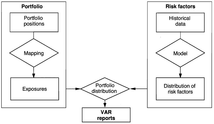
    • Risk Mapping
      • Introduction
      • Reasons for mapping
      • Stages of mapping
      • Selecting Core Instruments
      • Mapping with Principal Components
      • Mapping Positions to Risk Factors
      • A General Example of Risk Mapping
      • Example: Mapping with Factor Models
      • Example: Mapping with Fixed-Income Portfolios
      • Choice of Risk Factors
      • Mapping Complex Positions
      • Dealing with Optionality
    • VaR Methods
      • Delta-Normal
      • Historical Simulation
      • Monte Carlo Simulation
      • Comparison of Methods
    • Limitations of Risk Systems
      • Limitations of Risk Systems
      • 课堂练习
  • Introduction to Credit Risk
    • Settlement Risk
    • Overview of Credit Risk
      • Drivers of Credit Risk
      • Measurement of Credit Risk
    • Measuring Credit Risk
      • Credit Losses
  • Measuring Actuarial Default Risk
    • Credit Event
      • Credit Event
    • Default Rates
      • Credit Ratings
      • Historical Default Rates
      • Cumulative and Marginal Dafault Rates
      • Transition Probabilities
    • Recovery Rates
      • The Bankruptcy Processes
      • Estimates of Recovery Rates
  • Measuring Default Risk from Market Prices
    • Corporate Bond Prices
      • Spreads and Default Risk: Single Period
      • Spreads and Default Risk: Multiple Periods
      • Risk Premium
      • Cross-Section of Yield Spreads
      • Time Variation in Credit Spreads
    • Equity Prices
      • The Merton Model
      • Pricing Equity and Debt
      • Applying the Merton Model
      • A Detailed Example
      • 课堂练习
  • Credit Exposures
    • Credit Exposore by Instrument
      • Credit Exposore by Instrument
    • Distribution of Credit Exposure
      • Expected & Worse Exposure
      • Time Profile
    • Exposure Modifiers
      • Exposure Modifiers
    • Credit Risk Modifiers
      • Credit Risk Modifiers
  • Credit Derivatives and Structured Products
    • Introduction
    • Credit Default Swaps
      • Definition of CDS
      • Settlement
      • Pricing
      • Counterparty Risk
    • Other Contracts
      • CDS Variants
      • Total Return Swaps
      • Credit Spread Forwards and Option
    • Structured Products
      • Credit-Linked Notes
      • Collateralized Debt Obligations
  • Managing Credit Risk
    • Measuring the Distribution of Credit Losses
      • Measuring the Distribution of Credit Losses
    • Measuring Expected Credit Loss
      • Expected Loss over a Target Horizon
      • The Time Profile of Expected Loss
    • Measuring Credit VaR
      • Measuring Credit VaR
    • Portfolio Credit Risk Models
      • Approaches to Portfolio Credit Risk Models

---

Financial Risk Management Fundamental

Financial Risk

Definition

• Financial risk: prospect of financial gain or loss due to unforeseen changes in risk factors

• Market risks: arising from changes in market prices or rates
  Interest-rate risks, equity risks, exchange rate risks, commodity price risks, etc.

• Market vs. credit vs. operational risks

  • Credit risks: risks arising from possible default on contract
  • Op risks: risks from failure of people or systems

Contributory factors: volatile environment

• Stock market volatility

  • 23% fall in Dow Jones on Oct. 19, 1987
  • Dow Jones fell around 20% in July-Aug 1998
  • Massive falls in East Asian stock markets in 1998
  • 2015–16 Chinese stock market turbulence

• Exchange rate volatility

  • Problems of ERM (Exchange Rate Mechanism), peso, rouble, East Asia, etc.

• Interest rate volatility

  • US interest rates doubled over 1994

• Commodity market volatility

  • Electricity prices, etc.

Contributory factors: growth in trading activity

• Number of shares traded on NYSE grown from 3.5m in 1970 to 100m in 2000

• Turnover in FX markets grown from $1bn a day in 1965 to $1,210bn in April 2001

• Explosion in new financial instruments

• Securitization

• Growth of offshore trading

• Growth of hedge funds

• Derivatives

  • Few derivatives until early 1970s
  • FX futures (CME, 1972), equity calls (CBOT, 1973), interest-rate futures (1975)
  • Swaps and exotics (1980s)
  • Cat, credit, electricity, weather derivatives (1990s)
  • Daily notional principals negligible in early 1970s; up to nearly $2,800bn in April 2001

Contributory factors: advances in IT

• Huge increases in computational power and speed

  • Costs falling at 25-30% a year for 30 years

• Improvements in software

• Improvements in user-friendliness

  • E.g., in simulation software

• Risk measurers no longer constrained to simple back-of-the-envelope methods

---

Financial Risk Management before VaR

Risk measurement before VaR

• Gap analysis

• PV01 analysis

• Duration and duration-convexity analysis

• Scenario analysis

• Portfolio theory

• Derivatives risk measures

• Statistical methods, ALM, etc.

Gap Analysis

• Developed to get crude idea of interest-rate risk exposure

• Choose horizon, e.g., 1 year

• Determine how much of asset or liability portfolio re-prices in that period

  • Rate-sensitive assets / liabilities

• GAP = RS assets – RS liabilities

• Exposure is change in change in net interest income when interest rates change

  • $\Delta\text{NII}=\text{GAP}\times\Delta r$

• Pros

  • Easy to carry out
  • Intuitive

• Cons

  • Crude
  • Only applies to on-balance sheet IR risk
  • Looks at impact on income, not asset / liability values
  • Results sensitive to choice of horizon

PV01 Analysis

• Also applies to fixed income positions

• Addresses what will happen to bond price if interest rises by 1 basis point

• Price bond at current interest rates

• Price bond assuming rate rise by 1 bp

• Calculate loss as current minus prospective bond prices

Duration Analysis

• Another traditional approach to IR risk assessment

• Duration $D$ is weighted average of maturities of a bond’s cashflows,

  • weights are present values of each cashflow, divided by PV of all cashflows
  • $D=\frac{\sum_tt\times\text{PVCF}_t}{\sum_t\text{PVCF}_t}=\sum_tt\times\color{red}{\frac{\text{PVCF}_t}{\sum_t\text{PVCF}_t}}$

• Duration indicates sensitivity of bond price to change in yield:

  • $\frac{\Delta P}{\Delta y}=-PD\Longleftrightarrow\frac{\Delta P}{P}=-D\Delta y$

• Can approximate duration using simple algorithm as $(P_--P_+)/(2P_\Delta y)$, where $P_0$ is current price, $P_-$ is price when $\Delta y<0$, $P_+$ is price when $\Delta y>0$

• Duration is a linear function: duration of porfolio is sum of durations of bonds in portfolio

• Duration assumes $P-y$ relationship is linear when it is typically convex

• Duration ignores embedded options

• Duration analysis supposes that yield curve shifts in parallel

Convexity

• If duration takes a $P-y$ relationship as linear, convexity takes it as (approx) quadratic

• Convexity is the second order term in a Taylor series approximation
  $$\Delta P/P\approxeq-D\Delta y+(1/2)C(\Delta y)^2$$

• Convexity is defined as $C=(\Delta^2P/\Delta y^2)/P$

• Convexity term gives a refinement to the basic duration approximation

• In practice, convexity adjustment often small

• Convexity a valuable property

• Makes losses smaller, gains bigger

• Can approximate convexity as
  $$C\approxeq(P_-+P_+-2P_0)/(P_0\Delta y^2)$$

Pros and cons of duration-convexity

• Pros

  • Easy to calculate
  • Intuitive
  • Looks at values, not income

• Cons

  • Crude (only first-order approx, problems with non-parallel moves in spot rate curve, etc.)
  • Often inaccurate even with refinements (e.g., convexity)
  • Applies only to IR risks

Scenario Analysis

• 'What if' analysis – set out scenarios and work out what we gain/lose

• Select a set of scenarios, postulate cashflows under each scenario, use results to come to a view about exposure

• SA not easy to carry out

  • Much hinges on good choice of scenario
  • Need to ensure that scenarios do not involve contradictory or implausible assumptions
  • Need to think about interrelationships involved
  • Want to ensure that all important scenarios covered

• SA tells us nothing about probabilities

  • Need to use judgement to determine significance of results

• SA very subjective

• Much depends on skill and intuition of analyst

Portfolio Theory

• Starts from premise that investors choose between expected return and risk

  • Risk measured by std of portfolio return

• Wants high expected return and low risk

• Investor chooses portfolio based on strength of preferences for expected return and risk

  • Investor determines efficient portfolios, and chooses the one that best fits preferences

• Investor who is highly (slightly) risk averse will choose safe (risky) portfolio

• Key insight is that risk of any position is not its std, but the extent to which it contributes to portfolio std

  • Asset might have a high std, but contribute small risk, and vice versa

• Risk is measured by beta (\alert{why?}) – which depends on correlation of asset return with portfolio return

• High beta implies high correlation and high risk

• Low beta implies low correlation and low risk

• Zero beta implies no risk

• Ideally, looking for positions with negative beta

  • These reduce portfolio risk

• PT widely used by portfolio managers

• But runs into implementation problems

  • Estimation of beta highly problematic
  • Each beta is specific to data and portfolio
  • Need a long data set to get reliable result

• Practitioners often try to avoid some of these problems by working with `the' beta (as in CAPM)

  • But this often requires CAPM assumptions to hold
  • One market risk factor, etc.

• CAPM discredited (Fama-French, etc.)

Derivatives risk measures

• Can measure risks of derivatives positions by their Greeks

  • Delta $\Delta$ gives change in derivatives price for small change in underlying price
  • Gamma $\Gamma$ gives change in derivatives delta for small change in underlying price
  • Rho $\rho$ gives change in derivatives price for small change in interest rate
  • Theta $\Theta$ gives change in derivatives price for small change in time to maturity
  • Vega $\nu$ (\alert{which is not really a Greek letter}) gives change in derivatives price for small change in volatilty

• Use of Greeks requires considerable skill

• Need to handle different signals at the same time

• Risks measures only incremental

  • Work against small changes in exogenous factors
  • Can be Greek-hedged, but still be very exposed if there are large exogenous shifts
  • Hedging strategies require liquid markets, and can fail if market liquidity dries up (as in Oct 1987)

• Risk measures are dynamic

  • Can change considerably over time
  • E.g., gamma of ATM option goes to infinity

---

Value at Risk (VaR)

Value at Risk

• In late 1970s and 1980s, major financial institutions started work on internal models to measure and aggregate risks across institution

• As firms became more complex, it was becoming more difficult but also more important to get a view of firmwide risks

• Firms lacked the methodology to do so

  • Can't simply aggregate risks from sub-firm level

RiskMetrics

• Bestknown system is RiskMetrics developed by JP Morgan

• Supposedly developed by JPM staff to provide a '4:15' report to CEO, Dennis Weatherstone.

• What is maximum likely trading loss over next day, over whole firm?

• To develop this system, JPM used portfolio theory, but implementation issues were very difficult

• Staff had to

  • Choose measurement conventions
  • Construct data sets
  • Agree statistical assumptions
  • Agree procedures to estimate volatilities and correlations
  • Set up computer systems for estimation, etc.

• Main elements of system working by around 1990

• Then decided to use the '4:15' report

  • A one-day, one-page summary of the bank's market risk to be delivered to the CEO in the late afternoon (hence the ''4:15'')

• Found that it worked well

• Sensitised senior management to risk-expected return tradeoffs, etc.

• New system publicly launched in 1993 and attracted a lot of interest

• Other firms working on their systems

  • Some based on historical simulation, Monte Carlo simulation, etc.

• JPM decided to make a lower-grade version of its system publicly available

• This was RiskMetrics system launched in Oct 1994

  • Stimulated healthy debate on pros/cons of RiskMetrics, VaR, etc.

• Subsequent development of other VaR systems, applications to credit, liquidity, op risks, etc.

Portfolio theory and VaR

• PT interprets risk as std of portfolio return, VaR interprets it as maximum likely loss

  • VaR notion of risk more intuitive

• PT assumes returns are normal or near normal, whilst VaR systems can accommodate wider range of distributions

• VaR approaches can be applied to a wider range of problems

  • PT has difficulty applying to non-market risks, whereas VaR applies more easily to them

• VaR systems not all based on portfolio theory

  • Variance covariance systems are; others are not

Attractions of VaR

• VaR provides a single summary measure of possible portfolio losses

• VaR provides a common consistent measure of risk across different positions and risk factors

• VaR takes account of correlations between risk factors

Uses of VaR

• Can be used to set overall firm risk target

• Can use it to determine capital allocation

• Can provide a more consistent, integrated treatment of different risks

• Can be useful for reporting and disclosing

• Can be used to guide investment, hedging, trading and risk management decisions

• Can be used for remuneration purposes

• Can be applied to credit, liquidity and op risks

Criticisms of VaR

• VaR was warmly embraced by most practitioners, but not by all

• Concern with the statistical and other assumptions underlying VaR models

  • Hoppe and Taleb

• Concern with imprecision of VaR estimates

  • Beder

• Concern with implementation risk

  • Marshall and Siegel

• Concern with risk endogeneity

  • Traders might ‘game’ VaR systems
  • Write deep out-of-the-money options

• Uses of VaR as a regulatory constraint might destabilise financial system or obstruct good practice

• Concern that VaR might not be best risk measure

  • Limits of VaR, development of coherent risk measures

---

Advanced Risk Models: Univariate

Value-at-Risk (VaR)

• VaR is the maximum loss over a target horizon such that there is a low, prespecified probability that actual loss will be larger.

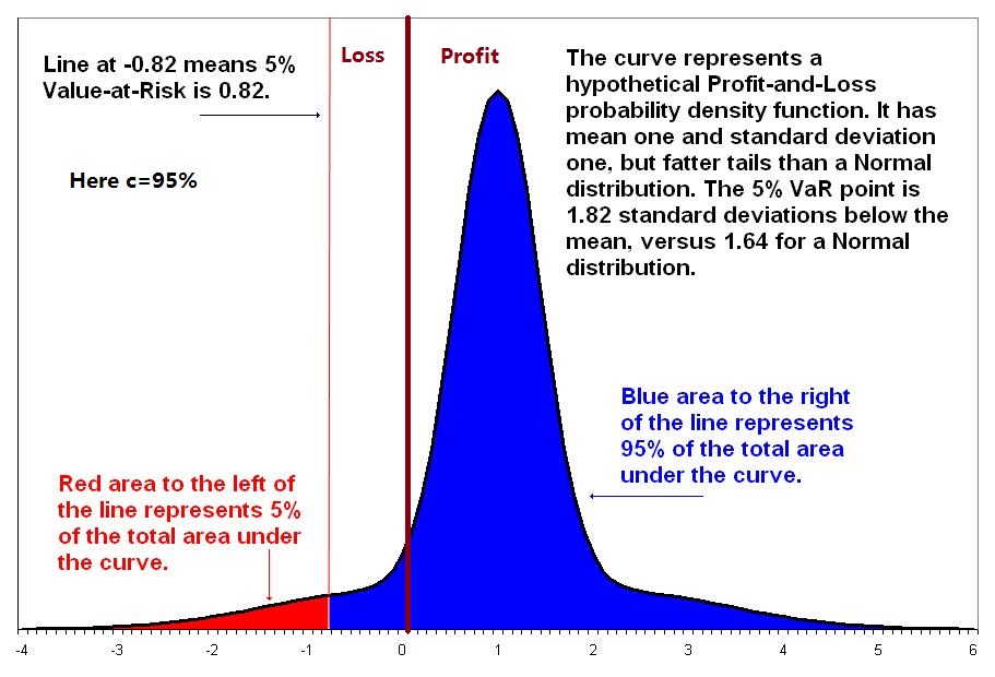
• Formula
  $$c=\int_{-VaR}^{\infty}f(x)dx$$ or,
  $$VaR_c(X)=\inf\left\{x\in\mathbb{R}^+:P(X<-x)\leq1-c\right\}$$

VaR Parameters: The Confidence Level (cl)

• VaR rises with confidence level (cl) at an increasing rate

VaR Parameters: The Holding Period (hp)

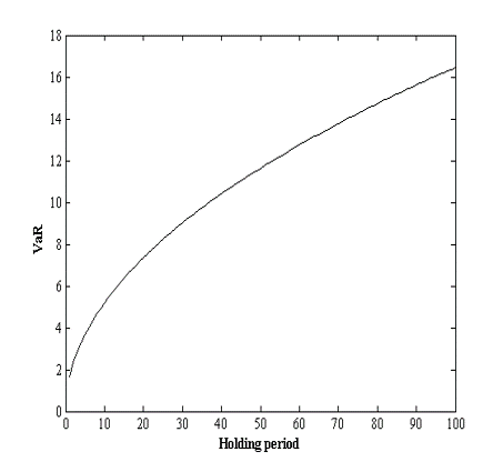
• If mean is zero, VaR rises with square root of holding period
• 'Square root rule': $\small VaR(T\text{ days})=VaR(1\text{ day})\times\sqrt{T}$
  • Daily innovations must be i.i.d. standard normal (why?)
• Empirical plausibility of SRR very doubtful (why?)

VaR Surface

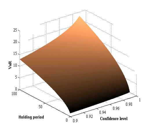
• VaR surface is much more revealing
• A single VaR number is just a point on the surface – doesn’t tell much
• With zero mean, get spike at high cl and high hp

Determine the Confidence Level

• High cl if we want to use VaR to set capital requirements

  • E.g., 99% under Basel

• Lower if we want to use VaR

  • to set position limits
  • for reporting/disclosure
  • for backtesting (we will discuss it later)

Determine the Holding Period

• Depends on investment/reporting horizons

• Daily common for cap market institutions

• 10 days (or 2 weeks) for banks under Basel

• Can depend on liquidity of market – hp should be equal to liquidation period

• Short hp makes it easier to justify assumption of unchanging portfolio

• Short hp preferable for model validation/backtesting requirements

  • Short hp means more data to use

Limitation of VaR

• VaR estimates subject to error

• VaR models subject to (considerable!) model risk

  • Beder

• VaR systems subject to implementation risk

  • Marshal and Siegel

• But these problems common to all risk measurement systems

VaR uninformative of tail losses

• VaR tells us most we can lose at a certain probability, i.e., if tail event does not occur

• VaR does not tell us anything about what might happen if tail event does occur

• Trader can spike firm by selling out of the money options

  • Usually makes a small profit, occasionally a very large loss
  • If prob of loss low enough, such a position appears to have no risk, but can be very dangerous

• Two positions with equal VaRs not necessarily equally risky, because tail events might be very different

• Solution to use more VaR information – estimate VaR at higher cl

VaR creates perverse incentives

• VaR-based decision calculus can be misleading, because it ignores low-prob, high-impact events

  • Events with probs less than VaR tail prob ignored

• Additional problems if VaR is used in a decentralized system

• VaR-constrained traders/managers have incentives to 'game' the VaR constraint

  • Sell out of the money options, etc.

VaR can discourage diversification

• VaR of diversified portfolio can be larger than VaR of undiversified one

• Example

  • 100 possible states, 100 assets, each making a profit in 99 (different) states, and a high loss in one
  • Diversified portfolio is certain to experience a high loss
  • Undiversified portfolio is not
  • Hence, VaR of diversified portfolio higher than VaR of undiversified one

VaR not subadditive

• A risk measure $\rho(\cdot)$ is subadditive if risk of sum is not greater than sum of risks
  $$\rho(A+B)\leq\rho(A)+\rho(B)$$

• Aggregating individual risks does not increase overall risk

• Important because: Adding risks together gives conservative (over-) estimate of portfolio risk – want bias to be conservative

• If risks not subadditive and VaR used to measure risk

  • Firms tempted to break themselves up to release capital
  • Traders on organized exchanges tempted to break up accounts
  • In both cases, problem of residual risk exposure

• Subadditivity is highly desirable

• But VaR is only subadditive if risks are normal or elliptical

• VaR not subadditive for arbitrary distributions

---

Coherent Measure of Risk

Coherent Risk Measures

• Let $X_1$ and $X_2$ be future values of two risky positions. A coherent measure of risk should satisfy the following axioms

  • Monotonicity: if $X_1\leq X_2$, $\rho(X_1)\leq\rho(X_2)$
  • Translation invariance: $\rho(X+k)=\rho(X)-k$
  • Homogeneity: $\rho(bX)=b\rho(X)$
  • Subadditivity: $\rho(X_1+X_2)\leq\rho(X_1)+\rho(X_2)$

• Homogeneity and Monotonicity imply convexity, which is important

• Translation invariance means that adding a sure amount to our end-period portfolio will reduce loss by amount added

Implications of coherence

• Any coherent risk measure is the maximum loss on a set of generalized scenarios

  • GS is set of loss values and associated probs

• Maximum loss from a subset of scenarios is coherent

• Outcomes of stress tests are coherent

  • Coherence theory provides a theoretical justification for stress testing!

• Coherence risk measures can be mapped to user’s risk preferences

• Each coherent measure has a weighting function $\phi(\cdot)$ that weights loss values

• $\phi(\cdot)$ can be linked to utility function (risk preferences)

• Can choose a coherent measure to suit risk preferences

Alternative Measures of Risk: CVaR

• The Conditional VaR (CVaR) is the expected loss, given a loss exceeding VaR
  $$CVaR=E[X|X<VaR_c(X)]=\frac{\int_{-\infty}^{VaR_c(X)}x\color{red}{f(x)}dx}{\color{red}{\int_{-\infty}^{VaR_c(X)}f(x)dx}}$$

• it is also called expected shortfall, tailed conditioal expectation, conditional loss, or expected tail loss

• VaR tells us the most we can lose if a tail event does not occur, CVaR tells us the amount we expect to lose if a tail event does occur

• CVaR is coherent

CVaR is better than VaR

• Tell us what to expect in bad states

  • VaR tells us nothing

• CVaR-based decision rule valid under more general conditions than a VaR-based one

  • CVaR rule valid under second-order stochastic dominance
  • VaR rule valid under first-order stochastic dominance
  • FOSD more stringent than SOSD

• CVaR coherent, and therefore always subadditive

• CVaR does not discourage risk diversification, VaR sometimes does

• CVaR-based risk surface always convex

  • Convexity ensures that portfolio optimization has a unique well-behaved optimum
  • Convexity also enables problems to be solved easily using linear programming methods

Alternative Measures of Risk: Worst-case scenario analysis

• This is the outcome of a worst-case scenario analysis (Boudoukh et al)

• Can consider as high percentile of distribution of losses exceeding VaR

  • Whereas CVaR is expected value of this distribution

• WCSA is also coherent, produces risk measures bigger than CVaR

Alternative Measures of Risk: SPAN

• Standard-Portfolio Analysis Risk (SPAN, CME)

• Considers 14 scenarios (moderate/large changes in vol, changes in price) + 2 extreme scenarios

• Positions revalued under each scenario, and the risk measure is the maximum loss under the first 14 scenarios plus 35% of the loss under the two extreme scenarios

• SPAN risk measure can be interpreted as maximum of expected loss under each of 16 probability measures, and is therefore coherent

Alternative Measures of Risk: Other Methods

• The Semistandard Deviation
  $$SG_L(X)=\sqrt{\frac{1}{N_L}\sum_{i=1}^N(x_i^-)^2}$$

• The Drawdown
  $$DD(X)=\frac{x^{\max}-x_t}{x^{\max}}$$

• Try to verify wether the following popular risk measures are coherent measures of risk or not

  • Standard deviation
  • VaR
  • CVaR
  • WCSA
  • SPAN

---

Backtesting

Backtesting

• Backtesting is the process to compare systematically the VaR forecasts with actual returns.

  • It should detect weaknesses in the models and point to areas for improvement
  • It is one of the reasons that bank regulators allow banks to use their own risk measures to determine the amount of regulatory capital

• Backtesting compares the daily VaR forecast with the realized profit and loss (P&L) the next day.

  • It is recorded as an exception if the actual loss is worse than the VaR
  • The risk manager counts the number if exceptions $x$ over a window with $T$ observations.

• Trading outcome

  • Actual portfolio
  • Hypothetical portfolio (no intraday trading, no fee income)
  • The Basel framework recommends using both hypothestical and actual trading outcomes in backtests

Preparing Data: Obtaining Data

• Need to obtain suitable P/L data

• Accounting (e.g., GAAP) data often inappropriate because of smoothing, prudence etc

• Want P/L data that reflect market risks taken

  • Need to eliminate fee income, bid-ask profits, P/L from other risks taken (e.g., credit risks), unrealised P/L, provisions against future losses

• Need to clean data or use hypothetical P/L data (obtained by revaluing periods from day to day)

Preparing Data: Draw up backtest chart

• Good to plot P/L data against risk bounds over time
• Chart good indicator of possible problems
  • over-estimation of risks
  • under-estimation of risks
  • bias
  • excessive smoothness in risk bounds, etc.

Preparing Data: Get to know data

• Draw up summary statistics

  • Mean, std, skewness, kutosis, min, max, etc.

• Draw up QQ charts

  • Plots of predicted vs. empirical quantiles

• Draw up charts of predicted vs. empirical probs

• Shape of these curves indicates whether supposed pdf fits the data – very useful diagnostic

Preparing Data: Standardise Data

• P/L data typically random

• Porfolios and dfs often change from day to day

• How to compare P/L data if underlying pdfs change?

• Good practice to map P/L data to predicted percentile

  • If observation falls 90% percentile of predicted P/L distribution, then mapped value is 0.90

• This standardizes data to make observations comparable given changes in pdf or porfolio

Measuring Exceptions

• Binomial Distribution

  • Probability mass function
    $$f(x)=\binom{T}{x}p^x(1-p)^{T-x},\ x=0,1,2,\dots,T$$
  • Mean: $pT$, Variance: $p(1-p)T$

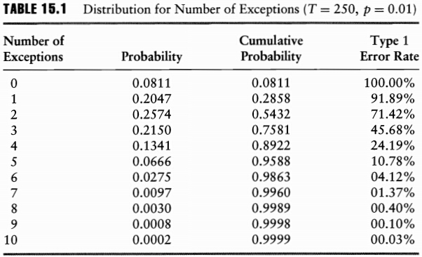
• Example: For instance, we want to know what is the probability of observing $x=0$ exceptions out of a sample of $T=250$ observations when the true probability is 1%. We should expect to observe $p\times T=2.5$ exceptions on average across many such samples. There will be, however, some samples with no exceptions at all simply due to luck. This probability is
  $$f(X=0)=\frac{T!}{x!(T-x)!}p^x(1-p)^{T-x}=\frac{250!}{1\times250!}0.01^00.99^{250}=0.081$$
  So, we would expect to observe 8.1% of samples with zero exceptions under the null hypothesis. We can repeat this calculation with different values for $x$. For example, the probability of observing eight exceptions is $f (X =8) = {250 \choose 8}0.01^8(0.99)^{242}=0.02\%$. Because this probability is so low, this outcome should raise questions as to whether the true probability is 1%.

• Normal Approximation
  $$z=\frac{x-pT}{\sqrt{p(1-p)T}}\sim N(0,1)$$

• Decision Rule for Backtests

  • Type 1 errors: kill the good guy
  • Type 2 errors: miss the bad guy
  • Power of a test is one minus the type 2 error rate
  • Most statistical tests fix the type 1 error rate, say at 5%, and structure the test so as to minimize the type 2 error rate, or maximize the test's power

Example

Consider a VaR measure over a daily horizon defined at the 99% level of confidence $c$. The window for backtesting is $T=250$ days.

• A higher cutoff point would lower the type 1 error rate
• It is more likely to miss VaR models that are misspecified with higher cutoff points

Basel Rule for Backtests

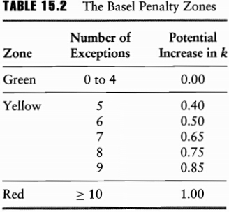
• The normal multiplier $k$ for capital charge is 3
• After an incursion into the yellow zone $k$ is increased to $4$ according to the table
• An incursion into the red zone generates an automatic, non-discretionary penalty

Evaluation of Backtesting

• Exception tests focus only on the frequency of occurrences

• It ignores the time pattern of losses

---

Advanced Risk Models: Multivariate

The Big Idea

Components of a Multivariate Risk Modeling Systems

• Risk system

  • portofolio position system
  • risk factor modeling system
  • aggregation system

• Describe joint movements in the risk factors

  • specify an analytical distribution
  • take the joint distribution from empirical observations

• Aggregation: VaR methods

  • delta-normal method
  • historical simulation method
  • Monte Carlo simulation method

---

Risk Mapping

Introduction

• Have assumed so far that each position has its own risk factor, which we model directly

  • Distinguish between positions and risk factors

• However, it is not always possible or desirable to model each position as having its own risk factor

• Might wish to map our positions onto some smaller set of risk factors

  • Might wish to map $n$ positions to $m$ ($<n$) risk factors

Reasons for mapping

• Might not have enough data on our positions

  • E.g., might have small runs of Emerging Market data
  • Map to risk factors for which we do have data

• Might wish to cut down on the dimensionality of our covariance matrices

  • This is important!
  • With $n$ positions, covariance matrix has $n(n+1)/2$ terms
  • As $n$ rises, covariance matrix becomes more unwieldy

• Need to keep dimensionality down to avoid computational problems too – rank problems, etc.

Stages of mapping

• Construct a set of benchmark instruments or factors

  • Might include key bonds, equities, etc.

• Collect data on their volatilities and correlations

• Derive synthetic substitutes for our positions, in terms of these benchmarks

  • This substitution is the actual mapping

• Construct VaR/CVaR of mapped porfolio

• Take this as a measure of the VaR/CVaR of actual portfolio

Selecting Core Instruments

• Usual approach to select key core instruments

  • Key equity indices, key zero bonds, key currencies, etc.

• Want to have a rich enough set of these proxies, but don’t want so many that we run into covariance matrix problems

• RiskMetrics core instruments

  • Equity positions represented by equivalent amounts in key equity indices
  • Fixed income positions by represented by combinations of cashflows of a limited number of maturities
  • FX positions represented by relevant amounts in `core' currenicies
  • Commodity positions represented by amounts of selected standardised futures positions

Mapping with Principal Components

• Can use PCA to identify key factors

• Small number of PCs will explain most movement in our data set

• PCA can cut down dramatically on dimensionality of our problem, and cut down on number of covariance terms

  • E.g., with 50 original variables, have $50(51)/2=1275$ separate covariance terms
  • With 3 PCs, have only 3 separate covariance terms

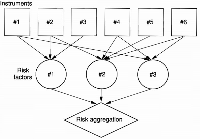
Mapping Positions to Risk Factors

• Most positions can be decomposed into primitive building blocks

• Instead of trying to map each type of position, we can map in terms of portfolios of building blocks

• Building blocks are

  • Basic FX
  • Basic equity
  • Basic fixed-income
  • Basic commodity

A General Example of Risk Mapping

• Replace each if the $N$ positions with a $K$ exposure on the risk factors. Define $x_{i,k}$ as the exposure of instruments $i$ to risk factor $k$
• Aggregate the $K$ exposures across the positions in the portfolio, $x_k=\sum_{i=1}^Nx_{i,k}$
• Derive the distribution of the portfolio return $R_{p,t+1}$ from the exposures and movements in risk factors, $\Delta f$, using one of the three VaR methods

Example: Mapping with Factor Models

• Decompose stock return $R_i=\alpha_i+\beta_i\times R_M+\epsilon_i$

  • a constant term (not important fot risk management purpose)
  • a component due to the market $R_M$
  • a residual term

• The portfolio return

  • Mean: $R_p=\sum_{i=1}^Nw_iR_i=\beta_pR_M+\sum_{i=1}^Nw_i\epsilon_i$
  • Variance: $V[R_p]=\beta^2_pV[R_M]+\sum_{i=1}^Nw_i^2V[\epsilon_i]$
  • For equally weighted portfolio: $\sum_{i=1}^Nw_i^2V[\epsilon_i]\rightarrow N\times\frac{V}{N^2}=\frac{V}{N}$
  • The mapping: $x_i$ on stock $i\rightarrow(x_i\beta_i)$ on index

• This approach is useful especially when there is no return history

Example: Mapping with Fixed-Income Portfolios

• Risk-free bond portfolio

  • maturity mapping: replace the current value of each bond by a position on a risk factor with the same maturity

  • duration mapping: maps the bond on a zero-coupon risk factor with a maturity equal to the duration of the bond

  • cash flow mapping: maps the current value of each bond payment on a zero-coupon risk factor with maturity equal to the time to wait for each cash flow

• Corporate bond portfolio

  • Decomposition: $y_i=z_j+s_k+\epsilon_i$
    

  • the movement in the value of bond price $i$:
    $$\Delta P_i=-DVBP_i\Delta y_i=-DVBP_i\Delta z_j-DVBP_i\Delta s_k-DVBP_i\Delta\epsilon_i$$

• the portfolio: $P=\sum_{i=1}^Nn_iP_i$

• aggregation:
  $$\begin{array}{lll} \Delta P&=&\sum_{i=1}^Nn_i\Delta P_i=-\sum_{i=1}^Nn_iDVBP_i\Delta y_i &=&-\sum_{j=1}^JDVBP_j^z\Delta z_j-\sum_{j=k}^KDVBP_k^s\Delta s_k-\sum_{i=1}^Nn_iDVBP_i\Delta \epsilon_i \end{array}$$

• Variance: $V[\Delta P]=\text{General Risk}+\sum_{i=1}^Nn^2_iDVBP_i^2V[\Delta\epsilon_i]$

• $x_i$ on bond $i\rightarrow(n_iDVBP_i)$ on $yield_j +(n_iDVBP_i)$ on $spread_k$

Choice of Risk Factors

It should be driven by the nature of the portfolio:

• portfolio of stocks that have many small positions well dispersed across sectors

• portfolios with a small number of stocks concentrated in one sector

• an equity market-neutral portfolio

• $\dots$

Mapping Complex Positions

• Complex positions are handled by apply financial engineering theory
• Reverse-engineer complex positions into portfolios of simple positions
• Map complex positions in terms of collections of synthetic simple positions
• Some examples, using FE/FI theory:
  • Coupon-paying bonds: can regard as portfolios of zeros
  • FRAs: equivalent to spreads in zeros of different maturities
  • FRNs: equivalent to a zero with maturity equal to period to next coupon payment (because it reprices at par)
  • Vanilla IR swaps: equivalent to portfolio long a fixed-coupon bond and short a FRN
  • Structured notes: equivalent to combinations of IR swaps and conventional FRNs
  • FX forwards: equivalent to spread between foreign currency bond and domestic currency bond
  • Commodity, equity and FX swaps: combinations of spread between forward/futures and bond position

Dealing with Optionality

• All these positions can be mapped with linear based mapping systems because of their being (close to) linear

• These approaches not so good with optionality

  • Non-linearity of options positions can lead to major errors in mapping

• With non-linearity, need to resort to more sophisticated methods, e.g., delta-gamma and duration-convexity

---

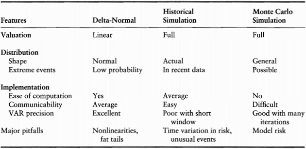
VaR Methods

Delta-Normal

• Assumption

  • portfolio exposures are linear
  • risk factors are jointly normally distributed

• The VaR

  • portfolio return is normally distributed
  • the portfolio variance: $\sigma^2(R_{p,t+1})=x_t'\Sigma_{t+1}x_t$
  • VaR is directly obtained from the standard normal deviate $\alpha$ that corresponds to the confidence level $c$:
    $$VaR=\alpha(c)\sigma(R_{p,t+1})$$
  • diversified VaR vs. undiversified VaR

• Advantages & Drawbacks

  • advantages: simple, closed-form, more precise, less sampling variability
  • drawbacks: can not account for nonlinear effects (option), underestimate the occurrence of large observations (normal assumption)

Historical Simulation

• The Idea: replays a ''tape'' of history to current positions

  • go back in time (e.g. over the past 250 days)
  • project hypothetical factor values using the factor movements
  • derive the portfolio values

• The VaR

  • current portfolio value as function of current risk factors: $P_t=P(f_{1,t},f_{2,t},\dots,f_{N,t})$
  • sampling factor movements from the historical distribution: $\Delta f_i^k=\{\Delta f_{i,1},\Delta f_{i,2},\dots,\Delta f_{i,t}\}$
  • construct hypothetical factor values: $f_i^k=f_{i,t}+\Delta f_i^k$
  • current portfolio value: $P^k=P(f_1^k,f_2^k,\dots,f_N^K)$
  • portfolio return: $R^k=\frac{P^k-P_t}{P_t}$
  • VaR is obtained from the difference between the average and the \textit{c}th quantile: $VaR=Ave(R_p)-R_p(c)$

• Advantages & Drawbacks

  • advantages: no specific distributional assumption, intuitive
  • drawbacks: its reliance on a short historical moving window to infer movements in market prices

Monte Carlo Simulation

• The Idea

  • is similar to the historical simulation method
  • the movements in risk factors are generated from a prespecified distribution: $\Delta f^k\sim g(\theta),\ k=1,\dots,K$
  • the risk manager needs to specify the marginal distribution of risk factors as well as their copula

• Advantages & Drawbacks

  • advantages: most flexible
  • drawbacks: computational burden, subject to model risk, sampling variability

• It should converge to the delta-normal VaR if all risk factors are normal and exposures are linear

Comparison of Methods

---

Limitations of Risk Systems

Limitations of Risk Systems

• Illiquid Assets

• Losses Beyond VaR

• Issues with Mapping

• Reliance on Recent Historical Data

• Procyclicality

• Crowded Trades

课堂练习

某交易组合是由价值300,000美元的黄金投资和价值500,000美元的白银投资构成，假定以上两资产的日波动率分别为1.8%和1.2%，并且两资产回报的相关系数为0.6，请问：（$\Phi(1.96)=0.975$）

(a) 交易组合10天展望期的97.5%VaR为多少？
(b) 投资分散效应减少的VaR为多少？

---

Introduction to Credit Risk

Settlement Risk

• Credit risk is the risk of an economic loss from the failure of a couterparty to fulfill its contractual obligations.

  • its effect is measured by the cost of replacing cash flow if the other party defaults
  • it requires constructing the distribution of default probabilities, of loss given default (LGD), and of credit exposures
  • traditionally, it is viewed as **presettlement risk, which arises during the life of the obligation

• Presettlement risk is the risk of loss due to the counterparty's failure to perform on an obligation during the life of the transaction

  • it includes the default on a loan or bond or failure to make required payment on a derivative transaction
  • it exists over long periods

• Settlement risk is due to the exchange of cash flow and is of a much shorter-term nature

  • it arises as soon as an institution makes the required payment and exists until the offsetting payment is received
  • the risk is greatest when payments occur in different time zones, especially for foreign exchange transactions where notional are exchanged in different currencies
  • it can be caused by counterparty default, liquidity constraints, or operational problems

• Status of a trade

  • Revocable: When the institution can still cancel the transaction without the consent of the counterparty
  • Irrevocable: After the payment has been sent and before payment from the other party is due
  • Uncertain: After the payment from the other party is due but before it is actually received
  • Settled: After the counterparty payment has been received
  • Failed: After it has been established that the counterparty has not made the payment

• Settlement risk occurs during the period of irrevocable and uncertain status (one to three days)

• Tools for settlement risk management

  • real-time-gross settlement (RTGS) system
  • netting agreements (bilateral netting, multilateral netting system / continuous-linked settlements )
  • contract for differences (CFDs)

---

Overview of Credit Risk

Drivers of Credit Risk

• Credit risk measurement systems attempt to quantify the risk of losses due to counterparty default

  • probability of default (PD)
  • credit exposure (CE)
  • loss given default (LGD) or recovery rate

• The borrower has the option to default, so the payment pattern is exactly equivalent to a short position in an option
  $$CE_t=\max(V_t,0)$$

---

Measurement of Credit Risk

• Measurement of Credit Risk

  • Notional amounts, adding up simple exposures
  • Risk-weighted amounts, adding up exposures with a rough adjustment for risk
  • Notional amounts combined with credit rating, adding up exposures adjusted for default probabilities
  • Internal portfolio credit models, integrating all dimensions of credit risk

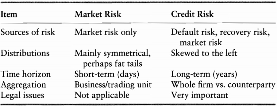
• Credit Risk versus Market Risk
  

---

Measuring Credit Risk

Credit Losses

Default mode: suppose all losses are due to the effect of defaults only.

The distribution of cresit losses (CLs) from a portfolio of $N$ instruments issued by different obligators can be described as
$$CL=\sum_{i=1}^Nb_i\times CE_i\times(1-f_i)$$

Measuring Actuarial Default Risk

Credit Event

Credit Event

Definition of **default by Standard & Pool's

Definition of **credit event by **International Swaps and Derivatives Association (ISDA)

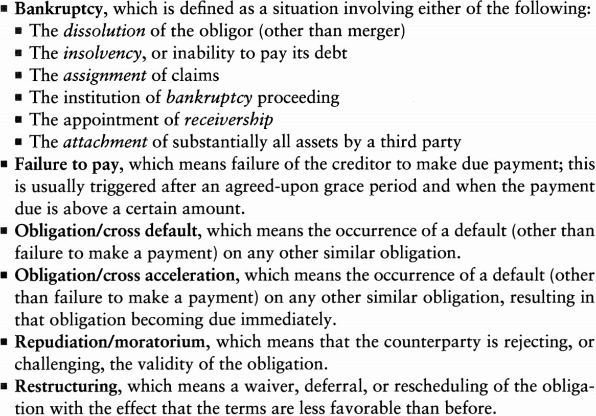
Other events sometimes included are

---

Default Rates

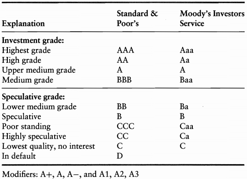
Credit Ratings

• A credit rating is an ''evaluation of creditworthiness'' issued by a credit rating agency (CRA).

• The major U.S. bond rating agencies are

  • Moody's Investors Service
  • Standard and Pool's (S&P)
  • Fitch Ratings

• Moody's definition of a credit rating

  
  
  
  

• Ratings represent objective (or actuarial) probabilities of default

  • published default frequencies can be used to convert ratings to default probabilities

• Ratings

  • investment grade
  • speculative grade, or below investment grade

• Classes & modifiers (also called notches)

---

• Accounting ratios & credit ratings
  
  
  
  

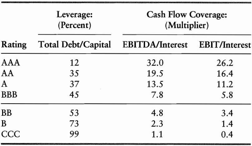
• Multiple Discriminant Analysis (MDA)

  • MDA constructs a linear combination of accounting data that provides the best fit with the observed states of default and non-default for the sample firms
  • $z-$score is an example of MDA

• $z-$score, variable used are:

  • working capital over other assets,
  • retained earnings over total assets,
  • EBIT over total assets,
  • market value of equity over total liabilities,
  • net sales over total assets.

---

Historical Default Rates

• The standard deviation of default probability (about 0.01%) for AA-rated credits is on the same of as the average (0.01%)
• Estimation of default rates for low probability events can be very imprecise

---

Cumulative and Marginal Dafault Rates

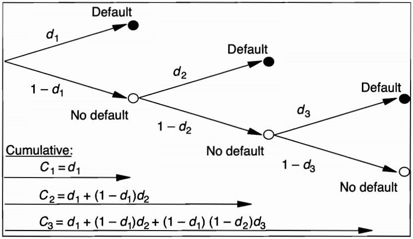
• Cumulative default rates measure the total frequency of default at any time between the starting date and year $T$, while marginal default rates measure default during year $T$

• Notations

  • $m[t+N|R(t)]$: the number of issuers rated $R$ at the end of year $t$ that default in year $T=t+N$
  • $n[t+N|]$: the number of issuers rated $R$ at the end of year $t$ that have not default by the beginning of year $T=t+N$

• Calculating rates

  %

  • Marginal Default Rate during Year $T$ : $d_N(R)=\frac{m[t+N|R(t)]} {n[t+N|R(t)]}$
  • Survival Rate: $S_N(R)=\prod_{i=1} ^N(1-d_i(R))$
  • Marginal Default Rate from Start to Year $T$ : $k_N(R)=S_{N-1} (R)d_N(R)$
  • Cumulative Default Rate: $C_N(R)=k_1(R)+k_2(R)+\cdots+k_N(R)=1-S_N(R)$
  • Average Default Rate: $C_N=1-\prod_{i=1} ^N(1-d_i)=1-(1-d)^N$
  • Average Default Rate for different compounding frequencies:
    $$C_N=1-(1-d^a)^N=1-(1-d^s/2)^{2N} \rightarrow1-e^{-d^cN}$$

---

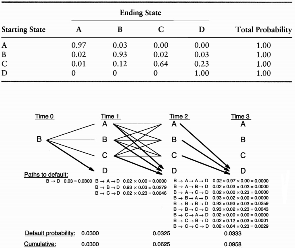
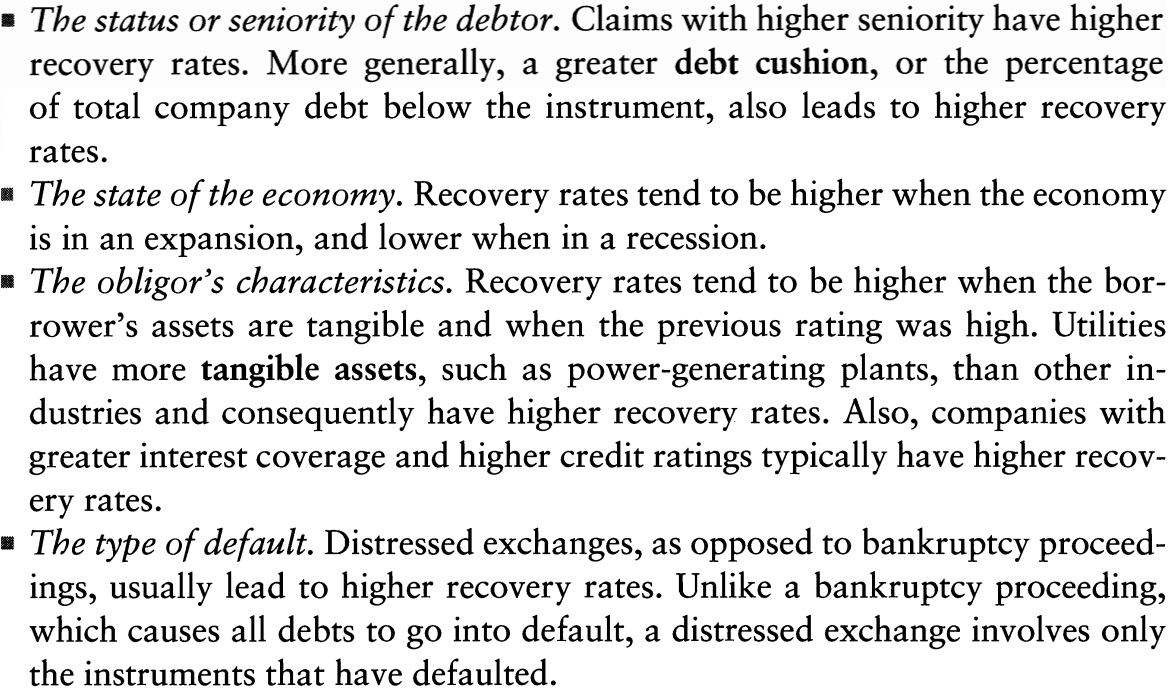
Transition Probabilities

Recovery Rates

The Bankruptcy Processes

Pecking order for a company's creditor:

---

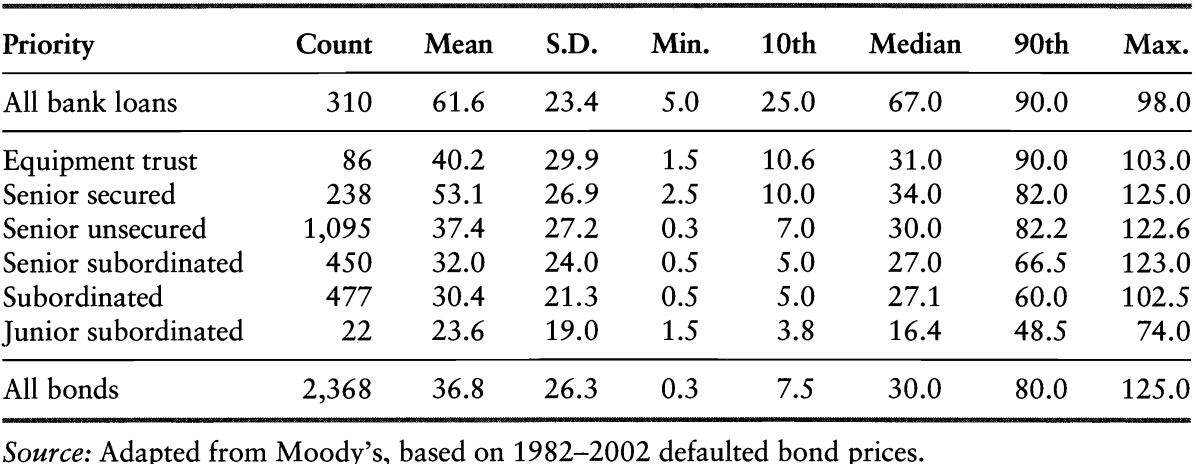
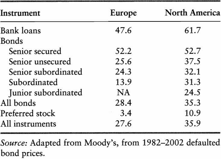
Estimates of Recovery Rates

The recovery rate depends on the following factors:

The recovery rate for corporate debt.

The legal environment is also a main driver of recovery rates.

• Trading prices of debt shortly after default can be used as an estimator of recovery rate, however, they are on average lower than the discounted recovery rates

  • clienteles for the two markets are different
  • risk premium in trading price

• An opportunity: buying the defaulted debt and working through the recovery process should create value

  • distress securities funds

---

Measuring Default Risk from Market Prices

Corporate Bond Prices

Spreads and Default Risk: Single Period

Suppose a bond has a single payment $100 in one period, the market-determined yield $y^*$ can be derived from its price $P^*$
$$P^*=\frac{\$100} {(1+y^*)}$$
We apply risk-neutral pricing:

$$P^*=\frac{\$100} {(1+y^*)} =\left[\frac{\$100 }{(1+y)} \right]\times(1-\pi)+\left[\frac{f\times\$100 }{(1+y) }\right]\times\pi$$
$$\Longrightarrow(1+y)=(1+y^*)[1-\pi(1-f)]\Longrightarrow\pi=\frac{1 }{1-f} \left[1-\frac{1+y }{1+y^*} \right]\Longrightarrow y^*\approx y+\pi(1-f)$$

---

Spreads and Default Risk: Multiple Periods

We compound interest rates and default rates over each period.Let $\pi^a$ be the average annual default rate.
$$P^*=\frac{\$100 }{(1+y^*)^T} =\left[\frac{\$100} {(1+y)^T }\right]\times(1-\pi^a)^T+\left[\frac{f\times\$100} {(1+y)^T }\right]\times[1-(1-\pi^a)^T]$$
$$\Longrightarrow(1+y)^T=(1+y^*)^T\{(1-\pi^a)^T+f[1-(1-\pi^a)^T]\}$$
If we use the cumulative default probability
$$\frac{1} {(1+y^*)^T} =\left[\frac{1} {(1+y)^T} \right]\times(1-\pi)+\left[\frac{f\times1} {(1+y)^T} \right]\times[1-(1-\pi)]$$
A very rough approximation:
$$\Longrightarrow\frac{1 }{(1+y^*)^T} =\left[\frac{1} {(1+y)^T} \right]\times[1-\pi(1-f)]\Longrightarrow y^*\approx y+(\pi/T)(1-f)$$

---

Risk Premium

In the previous analysis we assume risk neutrality. As a result, $\pi$ is a risk neutral measure, which is not necessarily equal to the objective, physical probability of default.

Assuming $\pi'$ and $y'$ be the physical probability of default and the discount rate. We have the following

$$P^*=\frac{\$100} {(1+y^*)} =\left[\frac{\$100} {(1+y')} \right]\times(1-\pi')+\left[\frac{f\times\$100} {(1+y')} \right]\times\pi'$$

$$\Longrightarrow y^*\approx y+\pi'(1-f)+rp$$

The risk premium ($rp$) must be tied to some meaure of bond riskiness as well as investor risk aversion. In addition, this premium may incorporate a **liquidity premium and tax effects.

---

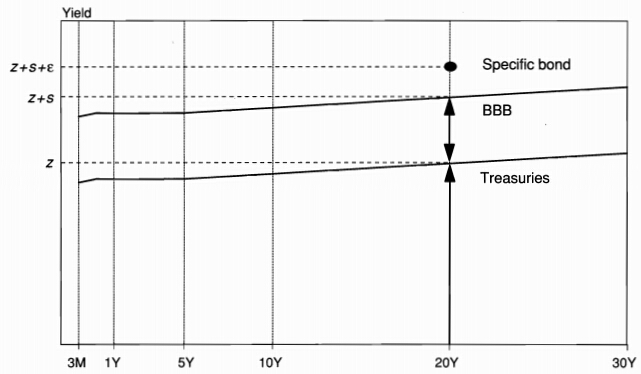
Cross-Section of Yield Spreads

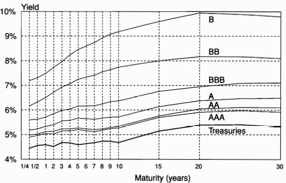
• The transition from Treasuries to AAA credit most likely reflects other factors, such as liquidity and tax effects, rather than actuarial credit risk

• We can use information in corporate bond yield to make inferences about credit risk

• Movements in corporate bond prices tend to \textit{lead changes in credit ratings

---

Time Variation in Credit Spreads

Part of default risk can be attributed to common credit risk factors such as

• General Economic conditions

  • growth
  • slow down

• Volatility

  • investors require more risk premium in a more volatile environment
  • liquidity may dry up

• The effect of volatility through an option channel

  • a callable bond = bond + (short) a call
  • the value of call increases in a more volatile environment

---

Equity Prices

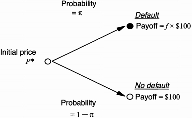
The Merton Model

• The Merton (1974) model views equity as akin to a call option on the assets of the firm, with an exercise price given by the face value of debt

• Consider a firm with total value $V$ that has one bond due in one period with face value $K$

  • equity can be viewed as a call option on the firm value with strike price equal to the face value of debt
    $$S_T=\max(V_T-K,0)$$
  • the current stock price embodies a forecast of default probability in the same way that an option embodies a forecast of being exercised
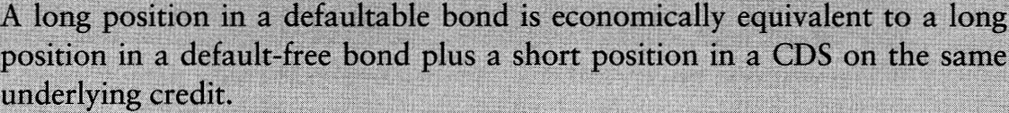
  • corporate debt can be viewed as risk-free debt minus a put option on the firm value
    $$B_T=V_T-S_T=\min(V_T,K)=K-\max(K-V_T,0)$$

---

Pricing Equity and Debt

Firm value follows the geometric Brownian motion
$$dV=\mu Vdt+\sigma vdz$$
The value of firm can be decompose in to the value of equity ($S$) and the value of debt ($B$). The corporate bond price is obtained as
$$B=F(V,t),\text{ }F(V,T)=\min(V,B_F),\text{ }B_F=K$$
The equity value is
$$S=f(V,t),\text{ }f(V,T)=\max(V-B_F,0)$$

Stock Valuation
$$S=\text{Call}=VN(d_1)-Ke^{-r\tau}N(d_2)$$
where $$d_1=\frac{\ln(V/Ke^{-r\tau})}{\sigma\sqrt{\tau}}+\frac{\sigma\sqrt{\tau}}{2},\text{ }d_2=d_1-\sigma\sqrt{\tau}$$

Firm Volatility
$$\sigma_V=(1/\Delta)\sigma_S(S/V)$$

Bond Valuation
$$B=\text{Risk-free bond}-\text{Put}\Longrightarrow B/Ke^{-r\tau}=N(d_2)+(V/Ke^{-r\tau})N(-d_2)$$

Risk-Neutral Dynamics of Default
$$1-N(d_2)=N(-d_2)$$

Pricing Credit Risk
$$\text{PD}=N[z]=N\{[\ln(K/V)-\delta\tau+0.5\sigma^2\tau]/[\sigma\sqrt{\tau}]\}$$

Credit Option Valuation
$$\text{Put}=Ke^{-r\tau}-\{Ke^{-r\tau}N(d_2)+V[1-N(d_1)]\}=-V[N(-d_1)]+Ke^{-r\tau}[N(-d_2)]$$

---

Applying the Merton Model

• the KMV approach: the company sells expected default frequencies (EDFs) for global firms

• Advantages

  • it relies on the price of equities, which are more actively traded than bonds
  • correlations between equity prices can generate correlations between bonds
  • it generates movements in EDFs that seems to \textit{lead changes in credit ratings

• Disadvantages

  • it can not be used to price sovereign credit risk
  • it relies on a static model of the firm's capital and risk structure
  • management could undertake new projects that increases not only the value if equity but also its volatility
  • the model fails to explain the magnitude of credit spreads we observe on credit-sensitive bonds

---

A Detailed Example

---

课堂练习

• [1] 假设某3年期企业债券每年支付7%的券息，每半年付息一次，收益率为5%（以每半年复利计）。所有期限的无风险债券的收益率均为4%（以每半年复利计）。假设违约事件可能每半年发生一次（刚好在债券每次付息之前），回收率为45%。请在以下假设下估计违约概率：

  • 在每个可能违约的日期，无条件违约概率均相同；

  • 在每个可能违约的日期之前无违约的条件下，发生违约条件概率均相同。
    
    
    

• [2] 请根据以下条件分析债券的违约概率和到期收益率：

  • 无风险利率为每年4%，某信用债券的收益率为每年6%。假设若该债券违约，回收率为70%。请估计该债券一年内发生违约的概率为多少？；

  • 某风险分析师尝试估计一个BB级债券的收益率。如果无风险利率为每年3.5%，BB级债券的违约概率为7%，违约损失率(Loss given default)为70%。请估计该债券的到期收益率。

---

Credit Exposures

Credit Exposore by Instrument

Credit Exposore by Instrument

• Credit exposure: $CE_t=\max(V_t,0)$

  • current exposure is the value of the asset at the current time $V_t$ if possitive
  • potential exposure represents the exposure on some future date, or set of dates

• Loans or Bonds

  • loans or bonds are balance sheet assets whose current and potential exposure basically is notional, or amount lent or invested
  • the exposure is also notional for receivables and trade credits, as the potential loss is the amount due

• Garantees

  • guarantees are off-balance-sheet contracts whereby the bank has underwritten, or agrees to assume, the obligations of a third party.
  • the exposure is the notional amount
  • it is irrevocable

• Commitments

  • Commitments are off-balance-sheet contracts whereby the bank commits to a future transaction that may result in creating a credit exposure at a \textit{future date
  • **irrevocable commitments vs. **revocable commitments

• Swaps or Forwards

  • Swaps or forwards contracts are off-balance-sheet items that can be viewed as irrevocable commitments to purchase or sell some asset on prearranged terms
  • the current and potential exposure will vary from zero to a large amount depending on movements in the driving risk factors
  • similar arrangement are **sale-repurchase (repos)

• Long Options

  • Options are off-balance-sheet items that may create many credit exposure
  • the current and potential exposure will vary from zero to a large amount depending on movements in the driving risk factors
  • there is no possibility for options to have negative values

• Short Options

  • the current and potential exposure for short options is zero because the bank writting the option can incur only a negative cash flow, assuming the option premium has been fully paid

---

Distribution of Credit Exposure

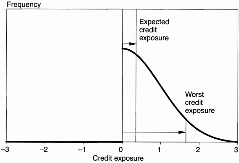
Expected & Worse Exposure

The expected credit exposure (ECE) is the expected value of the asset replacement value $x$, if positive, on a target date:
$$\text{ECE}=\int_{-\infty}^{\infty}x^+f(x)dx$$

The worse credit exposure (WCE) is the largest (worst) credit exposure at some level of confidence. It is implicitly defined as the value that is not exceeded at the given confidence level $p$:
$$1-p=\int_{\text{WCE}}^{\infty}f(x)dx$$

To model the potential credit exposure, we need to

• model the distribution of risk factors

• evaluate the instrument given these risk factors

• the process is identical to a market value at risk computation

• the aggregation takes place at the counterparty level if contracts are netted

---

Time Profile

The average expected credit exposure (AECE) is the average of the expected credit exposure over time, from now to maturity $T$:

$$\text{AECE}=\frac{1}{T}\int_{t=0}^T\text{ECE}_tdt$$

The average worst credit exposure (AWCE) is defined similarly:

$$\text{AWCE}=\frac{1}{T}\int_{t=0}^T\text{WCE}_tdt$$

---

Exposure Modifiers

Exposure Modifiers

Marking-to-Market (MTM)

• involves settling the variation in the contract value on a regular basis

  • it is called two-way marking to market if the treatment is symmetrical across the two counterparties
  • if one party settles losses only, it is called one-way marking to market

• Daily MTM reduces the current credit exposure to zero, however there is still potential exposure because the value of the contract would change before the next settlement. Potential exposure arises from:

  • the time interval between MTM periods
  • the time required for liquidating the contract when the counterparty defaults

• MTM introduces other types of risks

  • operational risk, which is due to the need to keep track of contract values and to make or receive payments daily
  • liquidity risk, because the institution now needs to keep enough cash to absorb variations in contract value

Margins

• Margins represent the cash or securities that must be advanced in order to open a position

  • the purpose of these funds is to provide a buffer against potential exposure
  • initial margin vs. maintenance margin

• Margins are set in relation to price volatility and to the type of position, speculation or hedging

  • margins increase for more volatile contracts
  • margins are typically lower for hedgers

Collateral

• OTC markets may allow posting securities as collateral instead of cash

  • the amount of collateral will exceed the funds owed by an amount known as haircut, which reflects both default risk and market risk.
  • collateral is typically managed within the International Swap and Derivatives Association (ISDA) credit support annex (CSA)

Exposure Limits

• Credit exposure can also be managed by setting position limits on the exposure to a counterparty
• To enforce limits, information on transactions must be centralized in middle-office systems
• These limits can also be set at the instrument level

Recouponing

• Recouponing refers to a clause in the contract requiring the contract to be marked to market at some fixed dates. It involves

  • exchanging cash to bring the MTM value to zero
  • resetting the coupon or the exchange rate to prevailing market value

Netting Arrangements

• It reduces the exposure to the net value for all the contracts covered by the netting agreement

• Nettings can be classified into three types:

  • payment netting involves the daily offsetting of several claims in the same currency
  • novation netting involves the cancellation of several contracts between the two parties, resulting in a replacement contract with new, net payments
  • close-out netting involves the cancellation of all transactions under the master agreement in the event of bankruptcy or any other specified default event

Other Modifiers

• third-party guarantees
• purchasing credit derivatives

---

Credit Risk Modifiers

Credit Risk Modifiers

• Credit triggers specify that if either counterparty's credit rating falls below a specified level, the other party has the right to have the swap cash settled

  • these are not exposure modifiers, but rather attempt to reduce the probability of default on that contract
  • these triggers are useful when the credit rating of a firm deteriorates slowly, because few firms jump directly from investment grade into bankruptcy

• Time puts, or mutual termination options, permit either counterparty to terminate the transaction unconditionally on one or more dates in the contract.

  • the feature decreases both the default risk and exposure
  • it allows one counterparty to terminate the contract if the exposure is large and the other party's rating starts to slip

• Triggers and put, which are types of contingent requirements, can cause serious trouble

---

Credit Derivatives and Structured Products

Introduction

• Credit derivatives provide an efficient mechanism to echange credit risk

  • credis risk can not be perfectly diversified for banks
  • banks can keep the loans on their books and to buy protection with credit derivatives

• Credit derivatives are over-the-counter contracts that allow credit risk to be exchanged across counterparties. They can be classified in terms of the following

  • The underlying credit, which can be a single entity (single name) or a group of entities (multiname)
  • The exercise conditions, which can be a credit event (such as default or rating downgrade, or an increase in credit spreads)
  • The payoff function, which can be a fixed amount or a variable amount with a linear or nonlinear payoff

---

Credit Default Swaps

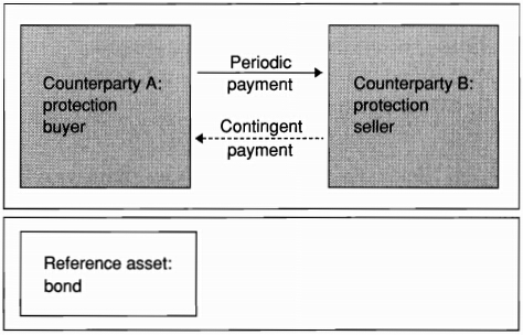
Definition of CDS

• In a credit default swap contract, a protection buyer (say A) pays a premium to the protection seller (say B), in exchange for payment if a credit evet occurs

  • the premium payment can be a lump sum or periodic
  • the contigent payment is triggered by a credit event (CE) on the underlying credit, say a bond issued by company Y

• A CDS is a option instead of a swap

  • the main difference from a regular option: the cost of a option is paid in installments instead of up front
  • if the cost is paid up front, the contract is called a default put option
  • the annual payment is referred as the CDS spread

• An example of CDS
  
  
  
  

• Most CDS contracts are quoted in terms of an annual spread, with the payment made on quarterly basis

• Default swaps are embedded in many financial products, for example:
  
  
  
  

---

Settlement

• The payment ($Q$) on default reflects the losses to the holders of the reference asset when the credit event occur. It takes a number of forms:

  • cash settlement, or a payment equal to the strike minusthe prevailing market value of the underlying bonds
  • physical settlement of the defaulted obligation in exchange for a fixed payment
  • a lump sum, or a fixed amount based on some pre-agreed recovery rate. (if the CE occurs, the recovery rate is set at 40%, leading to a payment of 60% of the notional)

• The payoff of a CDS is
  $$\text{Payment}=\text{Notional}\times Q\times I(\text{CE})$$

  • binary credit default swap: $Q=1$
  • with physical settlement, the contract defines a list of bond, which can trade at different prices but must be exchanged for their face value, that can be delivered (delivery option)
  • cash settlement can be conducted through an auction, which defines the recovery rate

---

Pricing

CDS contracts can be priced by considering the present value of the cash flows on each side of the contract.




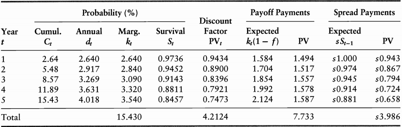
The value $V$ and the fair spread $s$ of the CDS contract should satisfy the following:

$$V=(\text{PV Payoff})-s(\text{PV Spread})=\left(\sum_{t=1}^Tk_t(1-f)PV_t\right)-s\left(\sum_{t=1}^TS_{t-1}PV_t\right)$$

The default probabilities used to price the CDS contracts must be risk-neutraal probabilities, not real-world probabilities.

---

Counterparty Risk

• A CDS does not eliminate credit risk entirely.

  • the protection buyer decreases exposure to the reference credit Y but assume new credit exposure to the CDS seller
  • correlation between the default risk of the underlying credit and of the couterparty is important

• A CDS is unfunded

  • unfunded: each party is resposible for making payments without recourse to other assets
  • ufunded: the protection seller makes a payment that could be used to settle any potential redit event

---

Other Contracts

CDS Variants

• The first-of-basket-to-default swap gives the protection buyer the right to deliver one and only one defaulted security out of a basket of selected securities

  • the contract will be more expensive than a single credit swap, all else kept equal
  • the price of protection also depends on the correlation between credit events

• With an $N$th-to-default swap, payment is triggered after $N$ defaults in the underlying portfolio, but not before

• CDS indices are widely used to track the performance of this market

  • the iTraxx indices cover the most liquid names in European and Asian credit markets
  • the North American and emerging markets are covered by the CDX indices

---

Total Return Swaps

A total return swap (TRS) is a contract where one party, called the protection buyer, makes a series of payments linked to the total return on a reference asset. In exchange, the protection seller makes a series of payments tied to a reference rate, such as the yield on an equivalent Treasury issue (or LIBOR ) plus a spread.

• TRS provides protection against credit risk in a mark-to-market (MTM) framework
• For the protection buyer, the TRS removes all the economic risk of the underlying asset without selling it
• Unlike a CDS, the TRS involves both creditrisk and market risk, the latter reflecting pure interest rate risk

---

Credit Spread Forwards and Option

In a credit spread forward contract, the buyer receives the difference between the credit spread at maturity and an agreed-upon spread, if positive. Conversely, a payment is made if the difference is negative. The payment is,
$$\text{Payment}=(S-F)\times \text{MD}\times\text{Notional}$$
Or, equivalently
$$\text{Payment}=[P(y+F,\tau)-P(y+S,\tau)]\times\text{Notional}$$
In a credit spread option contract, the buyer pays a premium in exchange for the right to put any increase in the spread to the option seller at a predefined maturity:
$$\text{Payment}=(S-K)^+\times \text{MD}\times\text{Notional}$$

---

Structured Products

Credit-Linked Notes

• Credit-linked notes (CLNs) are structured securities that combine a credit derivative with a regular bond

  • the buyer of protection transfers credit risk to an investor via an intermediary bond-issuing entity
  • the entity can be the buyer itself or a special-purpose vehicle (SPV)
  • this structure may carry a higher yield if the CDS spread is greater than the bond yield spread
  • this structure may also be attractive to investors who are precluded from investing directly in derivatives

---

Collateralized Debt Obligations

The waterfall structure of CDO

In this example, 80% of the capital structure is apportioned to tranche A, which has the highest credit rating of Aaa, using Moody’s rating, or AAA. It pays LIBOR + 45bp, for example. Other tranches have lower priorities and ratings. These intermediate, mezzanine, tranches are typically rated A, Baa, Ba, or B (A, BBB, BB, B, using S&P's ratings). For instance, tranche C would absorb losses from 3% to 10%. These numbers are called, respectively, the **attachment point and the detachment point.

---

Managing Credit Risk

Measuring the Distribution of Credit Losses

Measuring the Distribution of Credit Losses

Default mode (DM): considering only losses due to defaults instead of changges in market values

For a portfolio of $N$ conterparties, the credit loss (CL) is
$$\text{CL}=\sum_{i=1}^Nb_i\times\text{CE}_i\times\text{LGD}_i$$

The net replacement value (NRV)
$$\text{NRV}=\sum_{i=1}^N\text{CE}_i$$

• A typical distribution of credit profits & losses (P&L)
  
  
  
  

• The distribution of P&L is \textit{highly skewed to the left

  • similar to a short position in an option
  • Merton model:
    $$\text{A Risky bond}=\text{A risk-free bond}+\text{short an option}$$

• Major features

  • The Expected credit loss (ECL) represents the average credit loss. The pricing of the portfolio should be such that it covers the expected loss
  • The Unexpected credit loss (UCL) represents the loss that will not be exceeded at some level of confidence, typically 99.9%. Taking the deviation from the expected loss gives the unexpected credit loss. The institution should have enough equity capital to cover the unexpected loss.

The effect of correlations

• Correlations across default event $b_i$

• Correlations across default event and exposure

  • wrong-way trades: exposure is positively correlated with the probability of default
  • right-way trades occurs when the transaction is a hedge for the counterparty

---

Measuring Expected Credit Loss

Expected Loss over a Target Horizon

$$\begin{array}{lll} &&E[CL]=\int f(b,\text{CE},\text{LGD})(b\times\text{CE}\times\text{LGD})dbd\text{CE}d\text{LGD}\nonumber \end{array}$$

Assuming independency,

$$\begin{array}{lll} E[CL]&=&\left[\int f(b)(b)db\right]\left[\int f(\text{CE})(\text{CE})d\text{CE}\right]\nonumber\\ &&\left[\int f(\text{LGD})(\text{LGD})d\text{LGD}\right]\nonumber \end{array}$$

$$\begin{array}{lll} \Longrightarrow \text{ECL}=\Pr(\text{default})\times E[\text{CE}]\times E[\text{LGD}]\nonumber \end{array}$$

---

The Time Profile of Expected Loss

The present value of expected credit losses (PVECL):
$$\text{PVECL}=\sum_tE[\text{CL}_t]\times\text{PV}_t=\sum_t[k_t\times\text{ECE}_t\times(1-f)]\times\text{PV}_t$$

It can be simplified by adopting the average default probability and average exposure over the life of the asset:
$$\text{PVECL}_A=\text{Ave}[k_t]\times \text{Ave}[\text{ECE}_t]\times(1-f)\times\left[\sum_t\text{PV}_t\right]$$

An even simpler approach, when ECE is constant, considers the final maturity $T$ only, using the cumulative default rate $c_T$ and discount factor $\text{PV}_T$:
$$\text{PVECL}_F=c_T\times\text{ECE}\times(1-f)\times\text{PV}_T$$

---

Measuring Credit VaR

Measuring Credit VaR

• Credit VaR over a Target Horizon

  • At a given confidence level $c$, the worst credit loss (WCL) is defined such that
    $$1-c=\int_{WCL}^{\infty}f(x)dx$$
  • Credit VaR is defined as the unexpected credit loss at some confidence level, which is measured as the deviation from ECL:
    $$\text{Credit VaR}=\text{UCL}=\text{WCL}-\text{ECL}$$
  • It should be viewed as the economic capital to be held as a buffer against unexpected losses

• Using Credit VaR to Manage the Portfolio

  • rationales on trades: profitability vs. credit risk (credit VaR)
  • the marginal contribution to risk can be used to analyze the incremental effect of a proposed trade on the total portfolio risk
  • the marginal analysis can also help to establish the renumeration of capital required to support the position

---

Portfolio Credit Risk Models

Approaches to Portfolio Credit Risk Models

• Model Type

  • Top-down models group credit risks using single statistics. They aggregate many sources if risk viewed as homogeneous into an overall portfolio risk, without going into the details of individual transactions. It is appropriate for retail portfolios with large numbers of credits, but less so for corporate or sovereign loans.
  • Bottom-up models account for futures of each instrument. It is most similar to the structural decomposition of positions that characterizes market VaR systems. It is appropriate for corporate and capital market portfolios. It is also most useful for taking corrective action, because the risk structure can be reverse-engineered to modify the risk profile

• Risk Definitions

  • Default-mode models consider only outright default as a credit event
  • Mark-to-market (MTM) models consider changes in market values and ratings changes, including defaults

• Models of Default Probability

  • Conditional models incorporate changing macroeconomic factors into teh default probability through a functional relationship
  • Unconditional models have fixed default probabilities and tend to focus on borrower-or factor-specific information

• Models of Default Correlations

  • Structural Models explain correlations by the joint movements of assets
  • Reduced-form models explain correlations by assuming a particular functional relationship between the default probability and background factors

• Comparison of Credit Risk Models
  
  
  
  

---