专题： 期权拓展与应用

---

• 专题： 期权拓展与应用
  • 期权定价的拓展
    • 指数期权与货币期权
      • 指数期权
      • 中金所沪深300股指期权合约表
      • 指数期权的用途：组合保险}
      • 组合保险：例一
      • 组合保险：例二
      • 外汇期权
      • 期权性质：期权价格的下限
      • 期权性质：看跌期权-看涨期权平价关系
      • 定价
    • 期货期权
      • 概念
      • 期货期权的特性
      • 期权性质：看跌期权-看涨期权平价关系
      • 期权性质：期权价格的下限
      • 定价：二叉树
      • 定价：Black's Model
  • 期权定价的应用
    • Estimating Default Probability
      • The Merton Model
      • Pricing Equity and Debt
      • Applying the Merton Model
      • A Detailed Example
    • Real Options
      • An Alternative to the NPV Rule for Capital Investments
      • The Problem with using NPV to Value Options
      • Correct Discount Rates are Counter-Intuitive
      • General Approach to Valuation
      • Example (36.1)
      • Example (36.1)
      • Extension to Many Underlying Variables
      • Estimating the Market Price of Risk
      • Types of Options
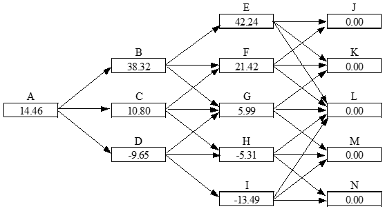
      • Example (Business Snapshot 36.1)
      • Example (page 795)
      • The Process for the Commodity Price
      • Estimating the Market Price of Risk Using CAPM (equation 36.2, page 792)
      • Valuation of Base Project; Fig 36.2
      • Valuation of Option to Abandon; Fig 36.3(No Salvage Value; No Further Payments)
      • Value of Expansion Option; Fig 36.4 (Company Can Increase Scale of Project by 20% for $2 million)
    • Appendix: Interest Rate Tree
      • Interest Rate Trees vs Stock Price Trees
      • Two-Step Tree Example
      • Alternative Branching Processes in a Trinomial Tree
      • Procedure for Building Tree
      • Example
      • Building the First Tree for the $\Delta t$ rate $R$
      • The First Tree
      • Shifting Notes
      • The Final Tree
      • Formulas for $\alpha$'s and $Q$'s}\footnotesize
  • Exotics
    • Types of Exotics
    • Packages
    • Perpetual American Options
    • Non-Standard American Options (page 598)
    • Gap Options
    • Forward Start Options (page 600)
    • Cliquet Option
    • Compound Option (page 600-601)
    • Chooser Option ``As You Like It'' (page 601-602)
    • Barrier Options (page 602-604)
    • Binary Options (page 604-605)
    • Lookback Options (page 605-607)
    • Shout Options (page 607)
    • Asian Options (page 608-609)
    • Exchange Options (page 609-610)
    • Basket Options (page 610-611)
    • Volatility and Variance Swaps
    • VIX Index (page 613-614)
    • How Difficult is it to Hedge Exotic Options?
    • Static Options Replication(Section 26.17, page 614-616)
    • Example
    • Using Static Options Replication

---

期权定价的拓展

指数期权与货币期权

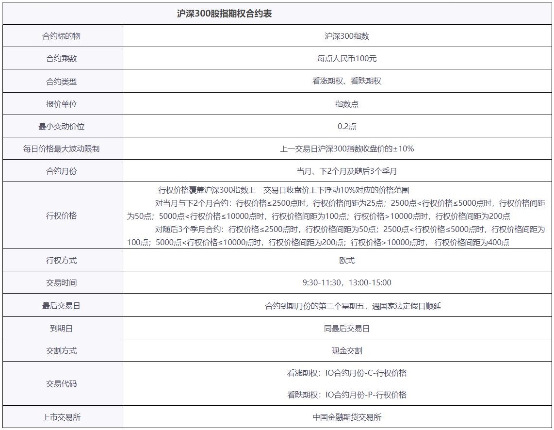
指数期权

• 指数期权：以股票指数作为标的

  • 上交所：50ETF期权（2017.12）、300ETF期权（2019.12）
  • 深交所：300ETF期权（2019.12）
  • 中金所：300股指期权（2019.12）

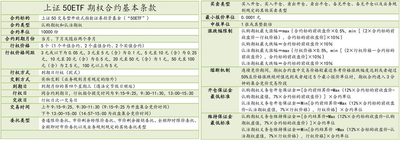
中金所沪深300股指期权合约表

指数期权的用途：组合保险}

• Suppose the value of the index is $S_0$ and the strike price is $K$

• If a portfolio has a $\beta$ of $1.0$, the portfolio insurance is obtained by buying $1$ put option contract on the index for each $100S_0$ dollars held

• If the $\beta$ is not $1.0$, the portfolio manager buys $\beta$ put option for each $100S_0$ dollars held

• In both cases, $K$ is chosen to give the appropriate insurance level

组合保险：例一

• Portfolio has a beta of 1.0
• It is currently worth $500,000
• The index currently stands at 1000
• What trade is necessary to provide insurance against the portfolio value falling below $450,000?

组合保险：例二

• Portfolio has a beta of 2.0

• It is currently worth $500,000 and index stands at 1000

• The risk-free rate is 12% per annum

• The dividend yield on both the portfolio and the index is 4%

• How many put option contracts should be purchased for portfolio insurance?

• Solution

  • If index rises to 1040, it provides a 40/1000 or 4% return in 3 months
  • Total return (incl. dividends) = 5%
  • Excess return over risk-free rate = 2%
  • Excess return for portfolio = 4%
  • Increase in Portfolio Value = 4+3−1=6%
  • Portfolio value=$530,000

• The Strike Price

Value of Index in 3 months	Expected Portfolio Value in 3 months ($)
1,080	570,000
1,040	530,000
1,000	490,000
960	450,000
920	410,000

• An option with a strike price of 960 will provide protection against a 10% decline in the portfolio value

外汇期权

• 外汇期权：以货币作为标的

  • 中国银行（期权宝）
  • 中国工商银行
  • 中国建设银行
  • 中国农业银行
  • 招商银行

• 范围远期合约 (Range-Forward Contract)

  • Have the effect of ensuring that the exchange rate paid or received will lie within a certain range
  • When currency is to be paid it involves selling a put with strike $K_1$ and buying a call with strike $K_2$ (with $K_2 > K_1$)
  • When currency is to be received it involves buying a put with strike $K_1$ and selling a call with strike $K_2$
  • Normally the price of the put equals the price of the call

期权性质：期权价格的下限

• 由以下等价关系得到：$c\geq\left(S_0e^{-qT}-Ke^{-rT}\right)^+$

  • 股票期初价格为$S_0$，股息收益率为$q$
  • 股票期初价格为$S_0e^{-qT}$，无股息

• 考虑投资组合A与投资组合B

  • 组合A： 一份欧式看涨期权+数量为$Ke^{-rT}$的现金
  • 组合B： $e^{-qT}$股股票，股息被再投资于股票

• 同理可得看跌期权价格下限：$p\geq\left(ke^{-rT}-S_0e^{-qT}\right)^+$

期权性质：看跌期权-看涨期权平价关系

• 考虑投资组合A与投资组合C

  • 组合A： 一份欧式看涨期权+数量为$Ke^{-rT}$的现金
  • 组合C： 一份欧式看跌期权+$e^{-qT}$股股票，股息被再投资于股票

• $c+Ke^{-rT}=p+S_0e^{-qT}$

• 美式期权
  $$S_0e^{-qT}-K\leq C-P\leq S_0-Ke^{-rT}$$

定价

• 偏微分方程
  $$\frac{\partial f}{\partial t}+(r-q)S\frac{\partial f}{\partial S}+\frac{1}{2}\sigma^2S^2\frac{\partial^2 f}{\partial S^2}=rf$$

• 定价公式

  • $c=S_0e^{-qT}N(d_1)-Ke^{-eT}N(d_2)$
  • $p=Ke^{-eT}N(-d_2)-S_0e^{-qT}N(-d_1)$
  • $d_1=\frac{\ln(S_0/K)+(r-q+\sigma^2/2)T}{\sigma\sqrt{T}},\text{ }d_2=d_1-\sigma\sqrt{T}$

• 风险中性定价

  • $c=e^{-rT}\left[F_0N(d_1)-KN(d_2)\right]$
  • $p=e^{-rT}\left[KN(-d_2)-F_0N(-d_1)\right]$
  • $F_0=S_0e^{(r-q)T}$

---

期货期权

概念

• 即期期权（spot options / options on spot）vs期货期权（futures options / options on futures）

• 期货期权

  • Referred to by the maturity month of the underlying futures
  • Usually they are American options
  • Expires on or a few days before the earliest delivery date of the underlying futures contract

期货期权的特性

• When a call futures option is exercised the holder acquires

  • A long position in the futures
  • A cash amount equal to the excess of the futures price at the time of the most recent settlement over the strike price
  • Payoff: $(F_T-K)^+$

• When a put futures option is exercised the holder acquires

  • A short position in the futures
  • A cash amount equal to the excess of the strike price over the futures price at the time of the most recent settlement
  • Payoff: $(K-F_T)^+$

• Potential advantages of futures options over spot options

  • Futures contracts may be easier to trade and more liquid than the underlying asset
  • Exercise of option does not lead to delivery of underlying asset
  • Futures options and futures usually trade on same exchange
  • Futures options may entail lower transactions costs

期权性质：看跌期权-看涨期权平价关系

• 欧式期货期权

  • European futures options and European spot options are equivalent when futures contract matures at the same time as the option
  • It is common to regard European spot options as European futures options when they are valued

• 考虑投资组合A与投资组合B

  • 组合A： 一份欧式看涨期权+数量为$Ke^{-rT}$的现金
  • 组合B： 一份欧式看跌期权+一份期货多头+数量为$F_0e^{-rT}$的现金

• $c+Ke^{-rT}=p+F_0e^{-rT}$

• 美式期权
  $$F_0e^{-rT}-K\leq C-P\leq F_0-Ke^{-rT}$$

期权性质：期权价格的下限

• 由看跌期权-看涨期权平价关系：$c+Ke^{-rT}=p+F_0e^{-rT}$

  • 看涨期权：$c\geq F_0e^{-rT}-Ke^{-rT}\Longrightarrow c\geq\left(\left(F_0-K\right)e^{-rT}\right)^+$
  • 看跌期权：$p\geq Ke^{-rT}-F_0e^{-rT}\Longrightarrow c\geq\left(\left(K-F_0\right)e^{-rT}\right)^+$

• 美式期权

  • 看涨期权：$C\geq(F_0-K)^+$
  • 看跌期权：$P\geq(K-F_0)^+$

定价：二叉树

• 与即期期权二叉树类似，但期初期货合约价格为0

• Growth Rates For Futures Prices

  • A futures contract requires no initial investment
  • In a risk-neutral world the expected return should be zero
  • The expected growth rate of the futures price is therefore zero
  • The futures price can therefore be treated like a stock paying a dividend yield of $r$

• $p=\frac{1-d}{u-d}$

定价：Black's Model

• 期货合约价值的漂移率

  • 风险中性：$e^{-ri\Delta t}\hat{E}[F_{i\Delta t}-F_0]=0,\ \forall i=1,2,\dots,N$
  • 漂移率为0：$\hat{E}[F_T]=F_0,\ \forall T$
  • $F$服从的随机微分方程：$dF=\sigma Fdz$

• 偏微分方程
  $$\frac{\partial f}{\partial t}+\frac{1}{2}\frac{\partial^2 f}{\partial F^2}\sigma^2F^2=rf$$

• Black's Model

  • $c=e^{-rT}\left[F_0N(d_1)-KN(d_2)\right]$
  • $p=e^{-rT}\left[KN(-d_2)-F_0N(-d_1)\right]$
  • $d_1=\frac{\ln(F_0/K)+\sigma^2T/2}{\sigma\sqrt{T}},\ d_2=d_1-\sigma\sqrt{T}$

• Application of Black's Model

  • Black's model is frequently used to value European options on the spot price of an asset
  • This avoids the need to estimate income on the asset

---

期权定价的应用

Estimating Default Probability

The Merton Model

• The Merton (1974) model views equity as akin to a call option on the assets of the firm, with an exercise price given by the face value of debt

• Consider a firm with total value $V$ that has one bond due in one period with face value $K$

  • equity can be viewed as a call option on the firm value with strike price equal to the face value of debt
    $$S_T=\max(V_T-K,0)$$
  • the current stock price embodies a forecast of default probability in the same way that an option embodies a forecast of being exercised
  • corporate debt can be viewed as risk-free debt minus a put option on the firm value
    $$B_T=V_T-S_T=\min(V_T,K)=K-\max(K-V_T,0)$$

Pricing Equity and Debt

Firm value follows the geometric Brownian motion
$$dV=\mu Vdt+\sigma vdz$$
The value of firm can be decompose in to the value of equity ($S$) and the value of debt ($B$). The corporate bond price is obtained as
$$B=F(V,t),\text{ }F(V,T)=\min(V,B_F),\text{ }B_F=K$$
The equity value is
$$S=f(V,t),\text{ }f(V,T)=\max(V-B_F,0)$$

Stock Valuation
$$S=\text{Call}=VN(d_1)-Ke^{-r\tau}N(d_2)$$
where $$d_1=\frac{\ln(V/Ke^{-r\tau})}{\sigma\sqrt{\tau}}+\frac{\sigma\sqrt{\tau}}{2},\text{ }d_2=d_1-\sigma\sqrt{\tau}$$

Firm Volatility
$$\sigma_V=(1/\Delta)\sigma_S(S/V)$$

Bond Valuation
$$B=\text{Risk-free bond}-\text{Put}\Longrightarrow B/Ke^{-r\tau}=N(d_2)+(V/Ke^{-r\tau})N(-d_2)$$

Risk-Neutral Dynamics of Default
$$1-N(d_2)=N(-d_2)$$

Pricing Credit Risk
$$\text{PD}=N[z]=N\{[\ln(K/V)-\delta\tau+0.5\sigma^2\tau]/[\sigma\sqrt{\tau}]\}$$

Credit Option Valuation
$$\text{Put}=Ke^{-r\tau}-\{Ke^{-r\tau}N(d_2)+V[1-N(d_1)]\}=-V[N(-d_1)]+Ke^{-r\tau}[N(-d_2)]$$

Applying the Merton Model

• the KMV approach: the company sells expected default frequencies (EDFs) for global firms

• Advantages

  • it relies on the price of equities, which are more actively traded than bonds
  • correlations between equity prices can generate correlations between bonds
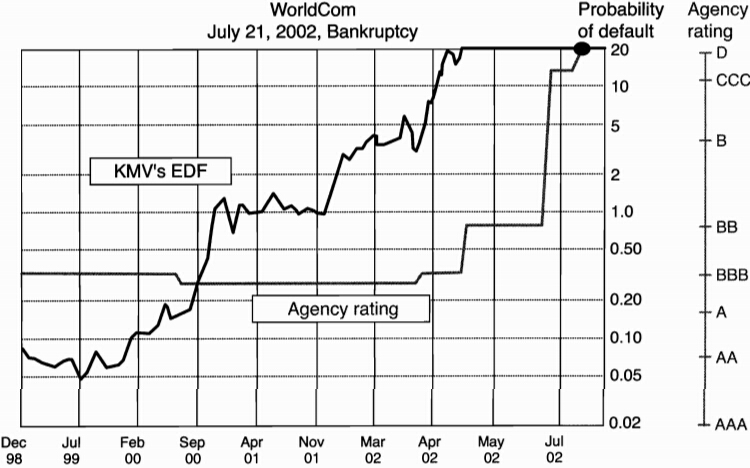
  • it generates movements in EDFs that seems to lead changes in credit ratings

• Disadvantages

  • it can not be used to price sovereign credit risk
  • it relies on a static model of the firm's capital and risk structure
  • management could undertake new projects that increases not only the value if equity but also its volatility
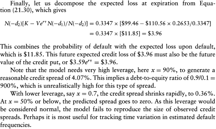
  • the model fails to explain the magnitude of credit spreads we observe on credit-sensitive bonds

A Detailed Example

---

Real Options

An Alternative to the NPV Rule for Capital Investments

• Define stochastic processes for the key underlying variables and use risk-neutral valuation

• This approach (known as the real options approach) is likely to do a better job at valuing growth options, abandonment options, etc than NPV

The Problem with using NPV to Value Options

• Consider the example from Chapter 13: risk-free rate =4%; strike price = $21

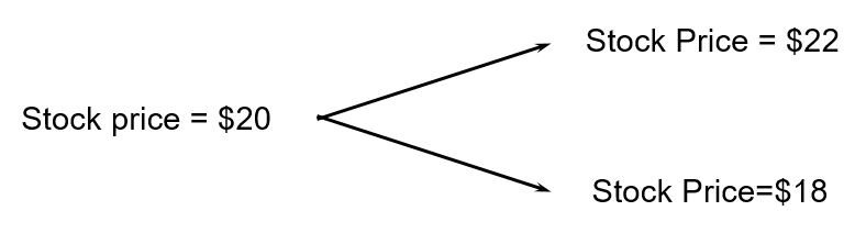
• Suppose that the expected return required by investors in the real world on the stock is 16%. What discount rate should we use to value an option with strike price $21?

Correct Discount Rates are Counter-Intuitive

• Correct discount rate for a call option is 42.6%

  • $c_u=\$1$, $c_d=\$0$, $c=\$0.663$, $p^*=0.7041$ if required expected return is $16\%$
  • $0.633e^{r\times0.25}=1\times0.7041\Longrightarrow r=42.58\%$

• Correct discount rate for a put option is –52.5%

General Approach to Valuation

• Assuming

  • The market price of risk for a variable $\theta$ is
    $$\lambda=\frac{\mu-r}{\sigma}$$
  • Suppose that a real asset depends on several variables $\theta_i,\ (i=1,2,\dots)$. Let $m_i$ and $s_i$ be the expected growth rate and volatility of $\theta_i$ so that
    $$d\theta_i/\theta_i=m_idt+s_idz_i$$

• We can value any asset dependent on a variable $\theta$ by

  • Reducing the expected growth rate of $\theta$ by $\lambda s$ where $\lambda$ is the market price of $\theta$-risk and $s$ is the volatility of $\theta$
  • Assuming that all investors are risk-neutral

Example (36.1)

The cost of renting commercial real estate in a certain city is quoted as the amount that would be paid per square foot per year in a new 5-year rental agreement. The current cost is $30 per square foot. The expected growth rate of the cost is 12% per annum, the volatility of the cost is 20% per annum, and its market price of risk is 0.3. A company has the opportunity to pay $1 million now for the option to rent 100,000 square feet at $35 per square foot for a 5-year period starting in 2 years. The risk-free rate is 5% per annum (assumed constant).

How to evaluate the option?

Example (36.1)

Define $V$ as the quoted cost per square foot of office space in 2 years. Assume that rent is paid annually in advance. The payoff from the option is

$$100,000A\max(V-35,0)$$

where $A$ is an annuity factor given by

$$A=1+\sum_{i=1}^41\times e^{-0.05\times i}=4.5355$$

The expected payoff in a risk-neutral world is therefore

$$100,000\times4.5355\times\hat{E}\left[\max(V-35,0)\right]=453,550\times\hat{E}\left[\max(V-35,0)\right]$$

According to the Black-Scholes formula, the value of the option is

$$453,550\left[\hat{E}[V]N(d_1)-35N(d_2)\right]$$

where

$$d_1=\frac{\ln\left[\hat{E}(V)/35\right]+0.2^2\times2/2}{0.2\sqrt{2}}$$

and

$$d_2=\frac{\ln\left[\hat{E}(V)/35\right]-0.2^2\times2/2}{0.2\sqrt{2}}$$

The expected growth rate in the cost of commercial real estate in a risk-neutral world is $m-\lambda s$, where $m$ is the real-world growth rate, $s$ is the volatility, and $\lambda$ is the market price of risk. In this case, $m=0.12$, $s=0.2$, and $\lambda=0.3$, so that the expected risk-neutral growth rate is 0.06, or 6%, per year. It follows that $\hat{E}[V]=30e^{0.06\times2}=33.82$. Substituting this in the expression above gives the expected payoff in a risk-neutral world as $1.5015 million. Discounting at the risk-free rate the value of the option is $1.5015e^{-0.05\times2}=\$1.3586$ million.

This shows that it is worth paying $1 million for the option.

Extension to Many Underlying Variables

• When there are several underlying variables qi we reduce the growth rate of each one by its market price of risk times its volatility and then behave as though the world is risk-neutral

• Note that the variables do not have to be prices of traded securities

Estimating the Market Price of Risk

• Contimuous CAPM:
  $$\mu-r=\frac{\rho\sigma}{\sigma_m}(\mu_m-r)$$

• According to the previous slides:
  $$\mu-r=\lambda\sigma$$

• The market price of risk:
  $$\lambda=\frac{\rho}{\sigma_m}(\mu_m-r)$$

Types of Options

• Abandonment

• Expansion

• Contraction

• Option to defer

• Option to extend life

Example (Business Snapshot 36.1)

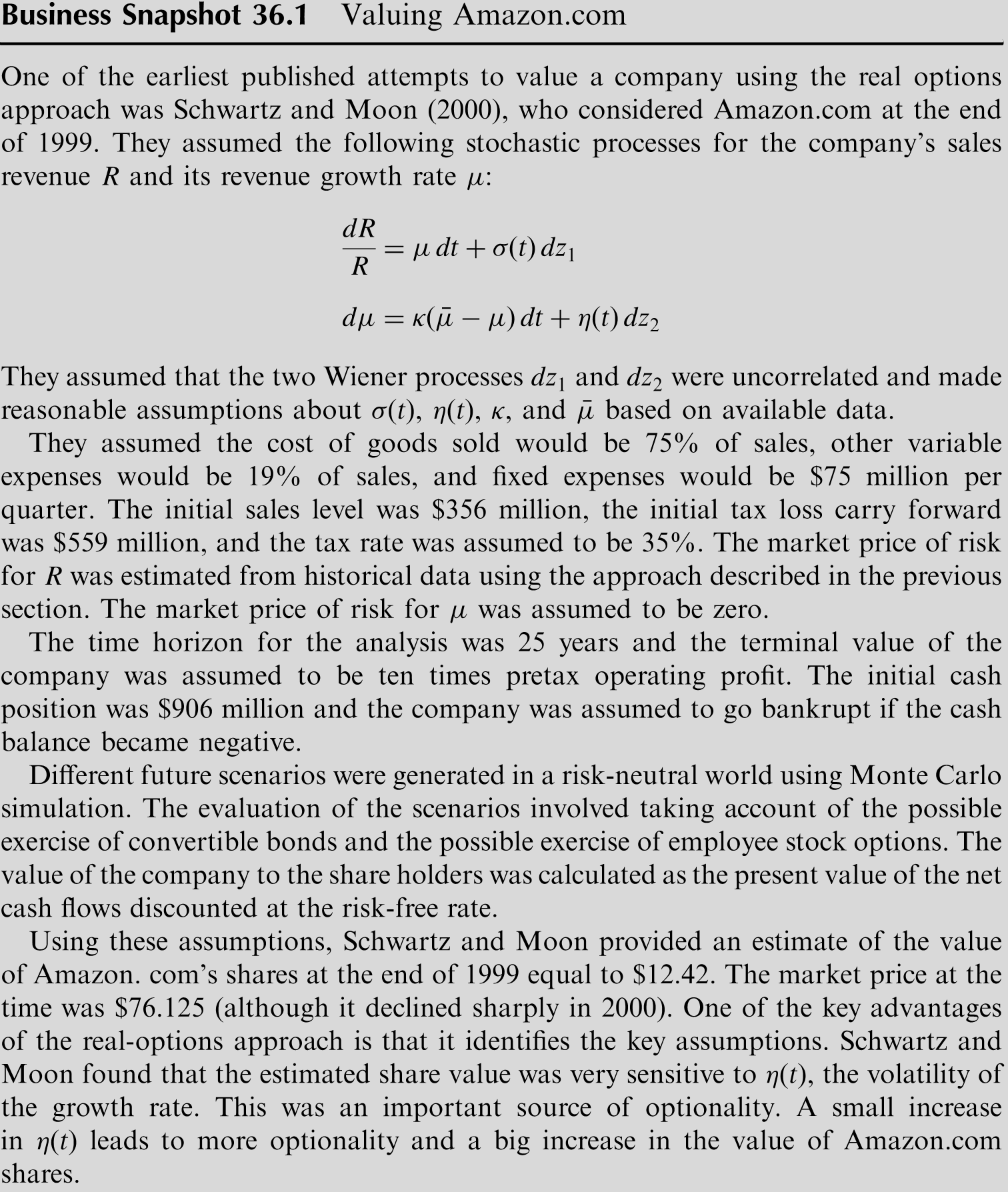
Example (page 795)

• A company has to decide whether to invest $15 million to obtain 6 million units of a commodity at the - rate of 2 million units per year for three years.
• The fixed operating costs are $6 million per year and the variable costs are $17 per unit.
• The spot price of the commodity is $20 per unit and 1, 2, and 3-year futures prices are $22, $23, and $24, respectively.
• The risk-free rate is 10% per annum for all maturities.

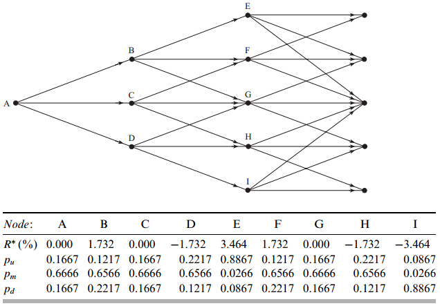
The Process for the Commodity Price

• We assume that this is
  $$d\ln(S)=[\theta(t)-a\ln(S)]dt+\sigma dz$$
  where $a=0.1$ and $\sigma=0.2$

• We build a tree as in Chapter 32 (Interest Rate Tree) and Chapter 35 (Energy and Commodity Derivatives)

Estimating the Market Price of Risk Using CAPM (equation 36.2, page 792)

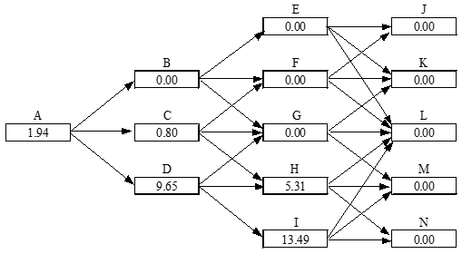
Node	A	B	C	D	E	F	G	H	I
$p_u$	0.1667	0.1217	0.1667	0.2217	0.8867	0.1217	0.1667	0.2217	0.0867
$p_m$	0.6666	0.6566	0.6666	0.6566	0.0266	0.6566	0.6666	0.6566	0.0266
$p_d$	0.1667	0.2217	0.1667	0.1217	0.0867	0.2217	0.1667	0.1217	0.8867

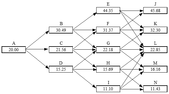
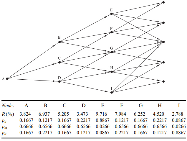
Valuation of Base Project; Fig 36.2

Node	A	B	C	D	E	F	G	H	I
$p_u$	0.1667	0.1217	0.1667	0.2217	0.8867	0.1217	0.1667	0.2217	0.0867
$p_m$	0.6666	0.6566	0.6666	0.6566	0.0266	0.6566	0.6666	0.6566	0.0266
$p_d$	0.1667	0.2217	0.1667	0.1217	0.0867	0.2217	0.1667	0.1217	0.8867

Valuation of Option to Abandon; Fig 36.3(No Salvage Value; No Further Payments)

Node	A	B	C	D	E	F	G	H	I
$p_u$	0.1667	0.1217	0.1667	0.2217	0.8867	0.1217	0.1667	0.2217	0.0867
$p_m$	0.6666	0.6566	0.6666	0.6566	0.0266	0.6566	0.6666	0.6566	0.0266
$p_d$	0.1667	0.2217	0.1667	0.1217	0.0867	0.2217	0.1667	0.1217	0.8867

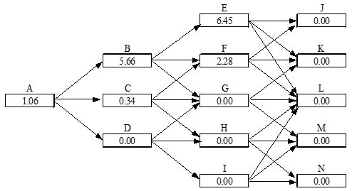
Value of Expansion Option; Fig 36.4 (Company Can Increase Scale of Project by 20% for $2 million)

Node	A	B	C	D	E	F	G	H	I
$p_u$	0.1667	0.1217	0.1667	0.2217	0.8867	0.1217	0.1667	0.2217	0.0867
$p_m$	0.6666	0.6566	0.6666	0.6566	0.0266	0.6566	0.6666	0.6566	0.0266
$p_d$	0.1667	0.2217	0.1667	0.1217	0.0867	0.2217	0.1667	0.1217	0.8867

Appendix: Interest Rate Tree

Interest Rate Trees vs Stock Price Trees

• The variable at each node in an interest rate tree is the $\Delta t$-period rate

• Interest rate trees work similarly to stock price trees except that the discount rate used varies from node to node

Two-Step Tree Example

Payoff after 2 years is $\max[100(r-0.11), 0]$, $p_u=0.25$; $p_m=0.5$; $p_d=0.25$; Time step=1yr

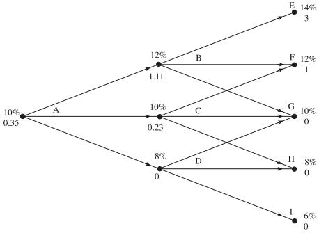
B: $(0.25\times3+0.50\times1+0.25\times0)e^{-0.12\times1}$

A: $(0.25\times1.11+0.50\times0.23+0.25\times0)e^{-0.10\times1}$

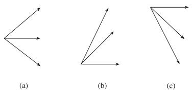
Alternative Branching Processes in a Trinomial Tree

Procedure for Building Tree

$$dr=[\theta(t)-ar]dt+\sigma dz$$

• [1] Assume $\theta(t ) = 0$ and $r (0) = 0$
• [2] Draw a trinomial tree for $r$ to match the mean and standard deviation of the process for $r$
• [3] Determine $\theta(t )$ one step at a time so that the tree matches the initial term structure

Example

Suppose that $\sigma=0.01$, $a=0.1$, and $\Delta t=1\text{yr}$. The zero-rate curve is given below.

Maturity	Zero Rate
0.5	3.430
1.0	3.824
1.5	4.183
2.0	4.512
2.5	4.812
3.0	5.086

Building the First Tree for the $\Delta t$ rate $R$

• Set vertical spacing: $$\Delta R=\sigma\sqrt{3\Delta t}$$

• Change branching when $j_{\max}$ nodes from middle where $j_{\max}$ is smallest integer greater than $0.184/(a\Delta t)$

• Choose probabilities on branches so that mean change in $R$ is $-aR\Delta t$ and S.D. of change is $\sigma\sqrt{\Delta t}$

The First Tree

Shifting Notes

• Work forward through tree

• Remember $Q_{ij}$ the value of a derivative providing a $1 payoff at node $j$ at time $i\Delta t$

• Shift nodes at time $i\Delta t$ by $\alpha_i$ so that the $(i+1)\Delta t$ bond is correctly priced

The Final Tree

Formulas for $\alpha$'s and $Q$'s}\footnotesize

To express the approach more formally, suppose that the $Q_{i,j}$ have been determined for $i\leq m\ (m>0)$. The next step is to determine $\alpha_m$ so that the tree correctly prices a zero-coupon bond maturing at $(m+1)\Delta t$. The interest rate at node $(m,j)$ is $\alpha_m+j\Delta R$,so that the price of a zero-coupon bond maturing at time $(m+1)\Delta t$ is given by
$$P_{m+1}=\sum_{j=-n_m}^{n_m}Q_{m,j}\exp[-(\alpha_m+j\Delta R)]\Delta t$$
where $n_m$ is the number of nodes on each side of the central node at time $m\Delta t$. The solution to this equation is
$$\alpha_m=\frac{\ln\sum_{j=-n_m}^{n_m}Q_{m,j}e^{-j\Delta R\Delta t}-\ln P_{m+1}}{\Delta t}$$
Once $\alpha_m$ has been determined, the $Q_{i,j}$ for $i=m+1$ can be calculated using
$$Q_{m+1,j}=\sum_{k}Q_{m,k}q(k,j)\exp[-(\alpha_m+k\Delta R)\Delta t]$$
where $q(k,j)$ is the probability of moving from node $(m,k)$ to node $(m+1,j)$ and the summation is taken over all values of $k$ for which this is nonzero.

---

Exotics

Types of Exotics

Packages	Barrier options
Perpetual American calls and puts	Binary options
Nonstandard American options	Lookback options
Gap options	Shout options
Forward start options	Asian options
Cliquet options	Options to exchange one asset for another
Compound options	Options involving several assets
Chooser options	Volatility and Variance swaps

Packages

• Portfolios of standard options
• Examples from Chapter 11: bull spreads, bear spreads, straddles, etc
• Often structured to have zero cost
• One popular package is a range forward contract (see Chapter 17)

Perpetual American Options

• Consider first a derivative that pays off $Q$ when $S = H$ for the first time and $S_0 < H$

• $f=Q(S/H)^\alpha\ (\alpha>0)$ satisfies the boundary conditions. It satisfies the differential equation
  $$\frac{\partial f}{\partial t}+(r-q)S\frac{\partial f}{\partial S}+\frac{1}{2}\sigma^2S^2\frac{\partial^2 f}{\partial S^2}=rf$$
  when
  $$(r-q)\alpha+\frac{1}{2}\alpha(1-\alpha)\sigma^2=r$$
  This has solutions $\alpha_1>0$ and $\alpha_2<0$

• The value of the derivative is therefore $Q(S/H)^{\alpha_1}$

• Consider next a perpetual American call option with strike price $K$

• If it is exercised when $S=H$ the value is $(H-K)(S/H)^{\alpha_1}$

• This is maximized when $H=K\alpha_1/(\alpha_1-1)$

• The value of the perpetual call is therefore
  $$\frac{K}{\alpha_1-1}\left(\frac{\alpha_1-1}{\alpha_1}\frac{S}{K}\right)^{\alpha_1}$$

• The value of a perpetual put is similarly
  $$\frac{K}{\alpha_2-1}\left(\frac{\alpha_2-1}{\alpha_2}\frac{S}{K}\right)^{-\alpha_2}$$

Non-Standard American Options (page 598)

• Exercisable only on specific dates (Bermudans)

• Early exercise allowed during only part of life (initial ``lock out'' period)

• Strike price changes over the life (warrants, convertibles)

Gap Options

• Gap call pays $S_T − K_1$ when $S_T > K_2$
• Gap put pays off $K_1 − S_T$ when $S_T < K_2$
• Can be valued with a small modification to BSM
  $$\text{Gap call}=S_0N(d_1)-K_1N(d_2)$$
  $$\text{Gap put}=K_1e^{-rT}N(-d_2)-S_0e^{-qT}N(-d_1)$$
  $$d_1=\frac{\ln(S_0/K_2)+(r-q+\sigma^2/2)T}{\sigma\sqrt{T}}$$
  $$d_2=d_1-\sigma\sqrt{T}$$

Forward Start Options (page 600)

• Option starts at a future time, $T_1$
• Implicit in employee stock option plans
• Often structured so that strike price equals asset price at time $T_1$
• Value is then $e^{-qT_1}$ times the value of similar option starting today

Cliquet Option

• A series of call or put options with rules determining how the strike price is determined
• For example, a cliquet might consist of 20 at-the-money three-month options. The total life would then be five years
• When one option expires a new similar at-the-money is comes into existence

Compound Option (page 600-601)

• Option to buy or sell an option

  • Call on call
  • Put on call
  • Call on put
  • Put on put

• Can be valued analytically

• Price is quite low compared with a regular option

Chooser Option ``As You Like It'' (page 601-602)

• Option starts at time $0$, matures at $T_2$
• At $T_1$ ($0 < T_1 < T_2$) buyer chooses whether it is a put or call
• This is a package!

At time $T_1$ the value is $\max(c,p)$. From put-call parity
$$p=c+e^{-r(T_2-T_1)}K-S_1e^{-q(T_2-T_1)}$$
The value at time $T_1$ is therefore
$$c+e^{-q(T_2-T_1)}\max\left(0,Ke^{-(r-q)(T_2-T_1)}-S_1\right)$$
This is a call maturing at time $T_2$ plus a position in a put maturing at time $T_1$.

Barrier Options (page 602-604)

• Option comes into existence only if stock price hits barrier before option maturity

  • "In" options

• Option dies if stock price hits barrier before option maturity

  • "Out" options

• Stock price must hit barrier from below

  • "Up" options

• Stock price must hit barrier from above

  • "Down" options

• Option may be a put or a call

• Eight possible combinations

• Parity Relations
  $$\begin{align} c=c_{ui}+c_{uo}, \text{ } p=p_{ui}+p_{uo} \nonumber\\ c=c_{di}+c_{do}, \text{ } p=p_{di}+p_{do} \nonumber \end{align}$$

Binary Options (page 604-605)

• Cash-or-nothing: pays $Q$ if $S_T > K$, otherwise pays nothing.

  • $\text{Value}=e^{-rT}QN(d_2)$

• Asset-or-nothing: pays $S_T$ if $S_T > K$, otherwise pays nothing.

  • $\text{Value}=S_0e^{-qT}QN(d_1)$

• Decomposition of a Call Option

  • Long: Asset-or-Nothing option
  • Short: Cash-or-Nothing option where payoff is $K$
  • $\text{Value}=S_0e^{-qT}QN(d_1)-e^{-rT}KN(d_2)$

Lookback Options (page 605-607)

• Floating lookback call pays $S_T – S_{\min}$ at time $T$ (Allows buyer to buy stock at lowest observed price in some interval of time)
• Floating lookback put pays $S_{\max}– S_T$ at time $T$ (Allows buyer to sell stock at highest observed price in some interval of time)
• Fixed lookback call pays $\max(S_{\max}−K, 0)$
• Fixed lookback put pays $\max(K −S_{\min}, 0)$
• Analytic valuation for all types

Shout Options (page 607)

• Buyer can `shout' once during option life

• Final payoff is either

  • Usual option payoff, $\max(S_T – K, 0)$, or
  • Intrinsic value at time of shout, $S_\tau – K$

• Payoff: $\max(S_T – S_\tau , 0) + S_\tau – K$

• Similar to lookback option but cheaper

Asian Options (page 608-609)

• Payoff related to average stock price

• Average Price options pay:

  • Call: $\max(S_{\text{ave}}-K,0)$
  • Put: $\max(K-S_{\text{ave}},0)$

• Average Strike options pay:

  • Call: $\max(S_T-S_{\text{ave}},0)$
  • Put: $\max(S_{\text{ave}}-S_T,0)$

• No exact analytic valuation

• Can be approximately valued by assuming that the average stock price is lognormally distributed

Exchange Options (page 609-610)

• Option to exchange one asset for another
• For example, an option to exchange one unit of $U$ for one unit of $V$
• Payoff is $\max(V_T – U_T, 0)$

Basket Options (page 610-611)

• A basket option is an option to buy or sell a portfolio of assets
• This can be valued by calculating the first two moments of the value of the basket at option maturity and then assuming it is lognormal

Volatility and Variance Swaps

• Volatility swap is agreement to exchange the realized volatility between time 0 and time T for a prespecified fixed volatility with both being multiplied by a prespecified principal

• Variance swap is agreement to exchange the realized variance rate between time 0 and time T for a prespecified fixed variance rate with both being multiplied by a prespecified principal

• Daily return is assumed to be zero in calculating the volatility or variance rate

• Variance Swap

  • The (risk-neutral) expected variance rate between times $0$ and $T$ can be calculated from the prices of European call and put options with different strikes and maturity $T$
  • For any value of $S^*$
    $$\begin{align} \hat{E}(\bar{V})&=&\frac{2}{T}\ln\frac{F_0}{S^*}-\frac{2}{T}\left[\frac{F_0}{S^*}-1\right]+\frac{2}{T}\int_{K=0}^{S^*}\frac{1}{K^2}e^{rT}p(K)dK\nonumber\\ &&+\frac{2}{T}\int_{K=S^*}^{\infty^*}\frac{1}{K^2}e^{rT}c(K)dK\nonumber \end{align}$$

• Volatility Swap

  • For a volatility swap it is necessary to use the approximate relation
    $$\hat{E}(\bar{\sigma})=\sqrt{\hat{E}(\bar{V})}\left\{1-\frac{1}{8}\left[\frac{var(\bar{V})}{\hat{E}(\bar{V})^2}\right]\right\}$$

VIX Index (page 613-614)

• The expected value of the variance of the S&P 500 over 30 days is calculated from the CBOE market prices of European put and call options on the S&P 500 using the expression for $\hat{E}(\bar{V})$
• This is then multiplied by 365/30 and the VIX index is set equal to the square root of the result

How Difficult is it to Hedge Exotic Options?

• In some cases exotic options are easier to hedge than the corresponding vanilla options (e.g., Asian options)
• In other cases they are more difficult to hedge (e.g., barrier options)

Static Options Replication(Section 26.17, page 614-616)

• This involves approximately replicating an exotic option with a portfolio of vanilla options
• Underlying principle: if we match the value of an exotic option on some boundary , we have matched it at all interior points of the boundary
• Static options replication can be contrasted with dynamic options replication where we have to trade continuously to match the option

Example

• A 9-month up-and-out call option an a non-dividend paying stock where $S_0 = 50$, $K = 50$, the barrier is $60$, $r = 10\%$, and $s = 30\%$

• Any boundary can be chosen but the natural one is

  • $c(S,0.75)=\max(S-50,0)$ when $S<60$
  • $c(60,t)=0$ when $0\leq t\leq 0.75$

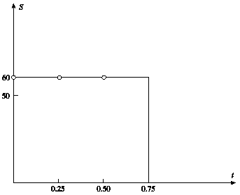
We might try to match the following points on the boundary

• $c(S,0.75)=\max(S-50,0)$ for $S<60$
• $c(60,0.50)=0$
• $c(60,0.25)=0$
• $c(60,0.00)=0$

We can do this as follows:

• +1.00 call with maturity 0.75 & strike 50

• –2.66 call with maturity 0.75 & strike 60

• +0.97 call with maturity 0.50 & strike 60

• +0.28 call with maturity 0.25 & strike 60

• This portfolio is worth 0.73 at time zero compared with 0.31 for the up-and out option

• As we use more options the value of the replicating portfolio converges to the value of the exotic option

• For example, with 18 points matched on the horizontal boundary the value of the replicating portfolio reduces to 0.38; with 100 points being matched it reduces to 0.32

Using Static Options Replication

• To hedge an exotic option we short the portfolio that replicates the boundary conditions
• The portfolio must be unwound when any part of the boundary is reached