L11 期权定价：B-S-M模型

---

• L11 期权定价：B-S-M模型
  • Wiener Processes and Itô's Lemma
    • Model the Dynamics of Stock Prices / Returns
      • ABC of Stochastic Processes
      • Variances & Standard Deviations
      • A Wiener Process
      • Norbert Wiener (诺伯特$\cdot$维纳)
      • Brownian Motion
      • Louis Bachelier (路易斯$\cdot$巴舍利耶)
      • Generalized Wiener Processes
      • Generalized Wiener Process
      • A Model for Stock Prices
    • It$\^{o}$'s lemma
      • Kiyosi It$\^{o}$ (伊藤清)
      • It$\^{o}$'s lemma
  • The Black-Scholes-Merton Model
    • The Stock Price Assumption
      • The Stock Price Assumption
      • Continuously Compounded Return
      • Volatility
    • The Black-Scholes-Merton Model
      • Black-Scholes-Merton: The Big Idea
      • The Derivation of the Black-Scholes-Merton Differential Equation
      • Black-Scholes-Merton Pricing for Options
      • Understanding Black-Scholes
    • Risk-Neutral Valuation
      • Risk-Neutral Valuation
  • Option Sensitivities: Greeks
    • Greeks
  • 课后阅读与练习
    • 课后阅读与练习

---

Wiener Processes and Itô's Lemma

Model the Dynamics of Stock Prices / Returns

ABC of Stochastic Processes

• Stochastic Processes

  • Describes the way in which a variable such as a stock price, exchange rate or interest rate changes through time
  • Incorporates uncertainties

• Example of Stochastic Processes

  • Each day a stock price: increases by $1 with probability 30, stays the same with probability 50%, reduces by $1 with probability 20%
  • Each day a stock price change is drawn from a normal distribution with mean $0.2 and standard deviation $1

• Markov Processes

  • In a Markov process future movements in a variable depend only on where we are, not the history of how we got to where we are
  • Is the process followed by the temperature at a certain place Markov?
  • We assume that stock prices follow Markov processes

• Weak-Form Market Efficiency

  • This asserts that it is impossible to produce consistently superior returns with a trading rule based on the past history of stock prices. In other words technical analysis does not work.
  • A Markov process for stock prices is consistent with weak-form market efficiency

Variances & Standard Deviations

• In Markov processes changes in successive periods of time are independent

• This means that variances are additive

• Standard deviations are not additive

• In our example it is correct to say that the variance is 100 per year.

• It is strictly speaking not correct to say that the standard deviation is 10 per year.

A Wiener Process

• Define $f(\mu,\nu)$ as a normal distribution with mean $\mu$ and variance $\nu$

• A variable $z$ follows a Wiener process if

  • The change in $z$ in a small interval of time $\Delta t$ is $\Delta z$
  • $\Delta z=\epsilon\sqrt{\Delta t}$ where $\epsilon\sim f(0,1)$
  • The values of $\Delta z$ for any $2$ different (non-overlapping) periods of time are independent

• Properties of a Wiener Process

  • Mean of $[z(T)-z(0)]$ is $0$
  • Variance of $[z(T)-z(0)]$ is $T$
  • Standard deviation of $[z (T )-z (0)]$ is $\sqrt{T}$

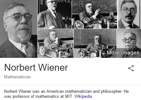
Norbert Wiener (诺伯特$\cdot$维纳)

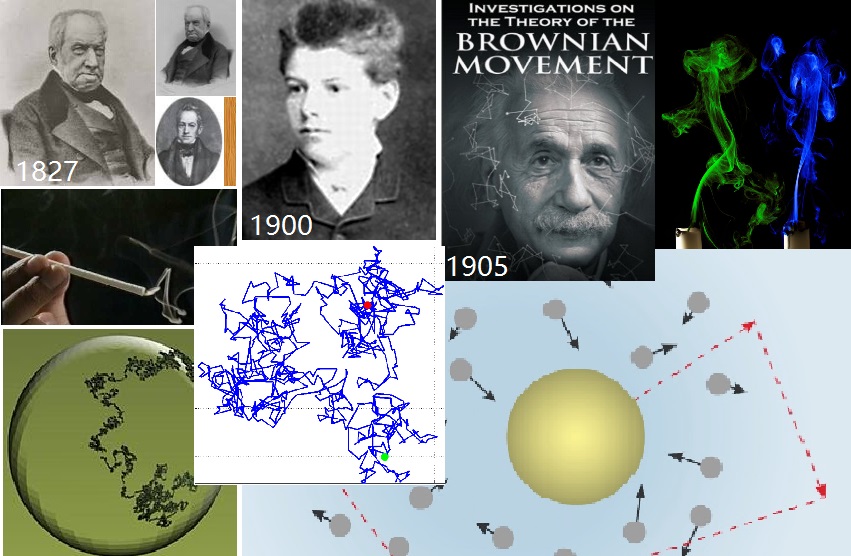
Brownian Motion

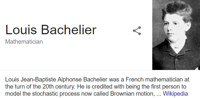
Louis Bachelier (路易斯$\cdot$巴舍利耶)

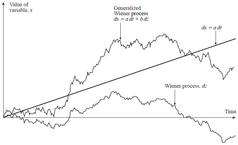
Generalized Wiener Processes

• A Wiener process has a drift rate (i.e. average change per unit time) of $0$ and a variance rate of $1$

• In a generalized Wiener process the drift rate and the variance rate can be set equal to any chosen constants
  $$\Delta x=a\Delta t+b\epsilon\sqrt{\Delta t}$$

  • Mean change in $x$ per unit time is $a$
  • Variance of change in $x$ per unit time is $b^2$

• Taking Limits

  • What does an expression involving $dz$ and $dt$ mean?
  • It should be interpreted as meaning that the corresponding expression involving $\Delta z$ and $\Delta t$ is true in the limit as $\Delta t$ tends to zero
  • In this respect, stochastic calculus is analogous to ordinary calculus

Generalized Wiener Process

A Model for Stock Prices

• It$\^{o}$ Process

  • In an It$\^{o}$ process the drift rate and the variance rate are functions of time
    $$dx=a(x,t) dt+b(x,t) dz$$
  • The discrete time equivalent $$\Delta x=a(x,t)\Delta t+b(x,t)\epsilon\sqrt{\Delta t}$$ is true in the limit as $\Delta t$ tends to zero

• A generalized Wiener process is not appropriate for stocks

  • For a stock price we can conjecture that its expected percentage change in a short period of time remains constant (not its expected actual change)
  • We can also conjecture that our uncertainty as to the size of future stock price movements is proportional to the level of the stock price

• Geometric Brownian Motion
  $$dS=\mu Sdt+\sigma Sdz$$

---

It$\^{o}$'s lemma

Kiyosi It$\^{o}$ (伊藤清)

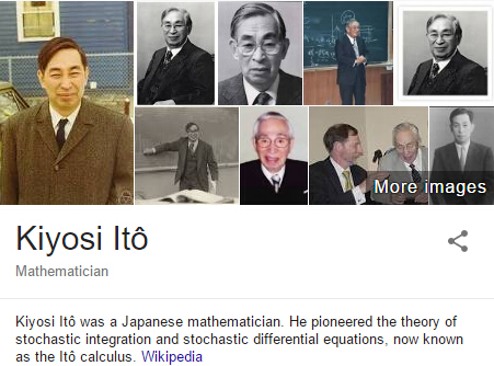
It$\^{o}$'s lemma

• If we know the stochastic process followed by $x$, It$\^{o}$'s lemma tells us the stochastic process followed by some function $G (x, t )$. When $dx=a(x,t) dt+b(x,t) dz$ then $$dG=\left(\frac{\partial G}{\partial x}a+\frac{\partial G}{\partial t}+\frac{1}{2}\frac{\partial^2 G}{\partial x^2}b^2\right)dt+\frac{\partial G}{\partial x}bdz$$

• Since a derivative is a function of the price of the underlying asset and time, It$\^{o}$'s lemma plays an important part in the analysis of derivatives

• Applications of It$\^{o}$'s Lemma to A Stock Price Process

  • Suppose the stock price process is $$dS=\mu Sdt+\sigma Sdz$$
  • For a function $G$ of $S$ and $t$ we have
    $$dG=\left(\frac{\partial G}{\partial S}\mu S+\frac{\partial G}{\partial t}+\frac{1}{2}\frac{\partial^2 G}{\partial S^2}\sigma^2S^2\right)dt+\frac{\partial G}{\partial S}\sigma Sdz$$

---

The Black-Scholes-Merton Model

The Stock Price Assumption

The Stock Price Assumption

• Consider a stock whose price is $S$

• In a short period of time of length $\Delta t$, the return on the stock is normally distributed:
  $$\frac{\Delta S}{S}\approx\phi(\mu\Delta t,\sigma^2\Delta t)$$

• So the price $S_T$ is lognormal distributed
  $$\ln S_T-\ln S_0\approx\phi\left[\left(\mu-\frac{\sigma^2}{2}\right)T,\sigma^2T\right]$$
  or
  $$\ln S_T\approx\phi\left[\ln S_0+\left(\mu-\frac{\sigma^2}{2}\right)T,\sigma^2T\right]$$

Continuously Compounded Return

• If $x$ is the realized continuously compounded return we have
  $$S_T=S_0e^{xT}$$
  $$x=\frac{1}{T}\ln\frac{S_T}{S_0}$$
  $$x\approx\left(\mu-\frac{\sigma^2}{2},\frac{\sigma^2}{T}\right)$$

• The Expected Return

  • The expected value of the stock price is $S_0e^{\mu T}$
  • The expected return on the stock is $\mu-\frac{\sigma^2}{2}$ not $\mu$
  • The reason is that, $\ln[E(S_T/S_0)]$ and $E[\ln(S_T/S_0)]$ are not the same

• $\mu$ vs. $\mu-\frac{\sigma^2}{2}$

  • $\mu$ is the expected return in a very short time, $\Delta t$, expressed with a compounding frequency of $\Delta t$
  • $\mu-\frac{\sigma^2}{2}$ is the expected return in a long period of time expressed with continuous compounding (or, to a good approximation, with a compounding frequency of $\Delta t$)

Volatility

• The Volatility

  • The volatility is the standard deviation of the continuously compounded rate of return in $1$ year
  • The standard deviation of the return in a short time period time $\Delta t$ is approximately $\sigma\sqrt{\Delta t}$
  • If a stock price is $50 and its volatility is 25% per year what is the standard deviation of the price change in one day?

• Estimating Volatility

  • Take observations $S_0, S_1,\dots,S_n$ at intervals of $t$ years (e.g. for weekly data $t = 1/52$)
  • Calculate the continuously compounded return in each interval as: $u_i=\ln\left(\frac{S_i}{S_{i-1}}\right)$
  • Calculate the standard deviation, $s$ , of the $u_i$'s
  • The historical volatility estimate is: $\hat{\sigma}=\frac{s}{\sqrt{\tau}}$

• Nature of Volatility

  • Volatility is usually much greater when the market is open (i.e. the asset is trading) than when it is closed
  • For this reason time is usually measured in ``trading days'' not calendar days when options are valued
  • It is assumed that there are $252$ trading days in one year for most assets

---

The Black-Scholes-Merton Model

Black-Scholes-Merton: The Big Idea

• The option price and the stock price depend on the same underlying source of uncertainty

• We can form a portfolio consisting of the stock and the option which eliminates this source of uncertainty

• The portfolio is instantaneously riskless and must instantaneously earn the risk-free rate

• This leads to the Black-Scholes-Merton differential equation

The Derivation of the Black-Scholes-Merton Differential Equation

• Stock price & derivative price
  $$\Delta S=\mu S\Delta t+\sigma S\Delta z$$
  $$\Delta f=\left(\frac{\partial f}{\partial S}\mu S+\frac{\partial f}{\partial t}+\frac{1}{2}\frac{\partial^2 f}{\partial S^2}\sigma^2S^2\right)\Delta t+\frac{\partial f}{\partial S}\sigma S\Delta z$$

• Set up a portfolio

  • derivative: $-1$
  • shares: $\Delta=+\frac{\partial f}{\partial S}$

• The value of the portfolio
  $$\Pi=-f+\frac{\partial f}{\partial S}S$$
  $$\Delta\Pi=-\Delta f+\frac{\partial f}{\partial S}\Delta S$$

Since the portfolio is risk-free, we have
$$\Delta\Pi=r\Pi\Delta t$$
$$-\Delta f+\frac{\partial f}{\partial S}\Delta S=r\left(-f+\frac{\partial f}{\partial S}S\right)\Delta t$$
So, the Black-Scholes-Merton Differential Equation is
$$\frac{\partial f}{\partial t}+rS\frac{\partial f}{\partial S}+\frac{1}{2}\sigma^2S^2\frac{\partial^2 f}{\partial S^2}=rf$$

• Any security whose price is dependent on the stock price satisfies the differential equation
• The particular security being valued is determined by the boundary conditions of the differential equation
• In a forward contract the boundary condition is $f= S-K$ when $t =T$
• The solution to the equation is
  $$f=S-Ke^{-r (T-t )}$$

Black-Scholes-Merton Pricing for Options

$$c=S_0N(d_1)-Ke^{-rT}N(d_2)$$
$$p=Ke^{-rT}N(-d_2)-S_0N(d_1)$$
where
$$d_1=\frac{\ln(S_0/K)+(r+\sigma^2/2)T}{\sigma\sqrt{T}}$$
$$d_2=\frac{\ln(S_0/K)+(r-\sigma^2/2)T}{\sigma\sqrt{T}}=d_1-\sigma\sqrt{T}$$

• Properties of Black-Scholes Formula
  • As $S_0$ becomes very large $c$ tends to $S_0 -Ke^{-rT}$ and p tends to zero
  • As $S_0$ becomes very small $c$ tends to zero and $p$ tends to $Ke^{-rT}-S_0$
  • What happens as $\sigma$ becomes very large?
  • What happens as $T$ becomes very large?

Understanding Black-Scholes

The formula
$$c=e^{-rT}N(d_2)\left(S_0e^{rT}N(d_1)/N(d_2)-K\right)$$

• $e^{-rT}$: Discount rate
• $N(d_2)$: Probability of exercise
• $e^{rT}N(d_1)/N(d_2)$: Expected percentage increase in stock price if option is exercised
• $K$: Strike price paid if option is exercised

---

Risk-Neutral Valuation

Risk-Neutral Valuation

• Risk-Neutral Valuation

  • The variable $\mu$ does not appear in the Black-Scholes-Merton differential equation
  • The equation is independent of all variables affected by risk preference
  • The solution to the differential equation is therefore the same in a risk-free world as it is in the real world
  • This leads to the principle of risk-neutral valuation

• Applying Risk-Neutral Valuation

  • [1] Assume that the expected return from the stock price is the risk-free rate
  • [2] Calculate the expected payoff from the option
  • [3] Discount at the risk-free rate

---

Option Sensitivities: Greeks

Greeks

The Taylor Expansion
$$df=\frac{\partial f}{\partial S}dS+\frac{1}{2}\frac{\partial^2 f}{\partial S^2}dS^2+\frac{\partial f}{\partial r}dr+\frac{\partial f}{\partial r^*}dr^*+\frac{\partial f}{\partial \sigma}d\sigma+\frac{\partial f}{\partial \tau}d\tau+\dots$$

• Delta: $\Delta=\frac{\partial f}{\partial S}$
• Gamma: $\Gamma=\frac{\partial^2 f}{\partial S^2}$
• Vega: $\Lambda=\frac{\partial f}{\partial \sigma}$
• Rho: $\rho=\frac{\partial f}{\partial r}$
• Theta: $\Theta=\frac{\partial f}{\partial t}=-\frac{\partial f}{\partial \tau}$

---

课后阅读与练习

课后阅读与练习

• 课后阅读：教材第十一章第三节、十二章第一节、第六章、第七章相关内容

• 练习

  • 教材pp186：7，10
  • 扫码做题